2 Chapter 2: Basics of SFA for cross-sectional data

2.1 Exercise 2.1 Data Import

This exercise demonstrates importing the data file cowing.xlsx in Python using the Pandas read_excel function. After importing, we display the first two lines and the last line of the data set.

import pandas as pd
import numpy as np 

data = pd.read_excel('cowing.xlsx', index_col=[0]) # use the first column of the excel file as the index
data.columns = ['lnY','lnK','lnF', 'lnL', 'P_K', 'P_F', 'P_L']
data.index.name = 'Utility' # The index column is the utility firm
display(data.head(2))
display(data.tail(1))

	lnY	lnK	lnF	lnL	P_K	P_F	P_L
Utility
1	6.955593	16.312510	16.348255	11.849398	0.0338	0.197	1.590003
2	7.255591	16.916638	16.507648	11.338572	0.0350	0.254	2.050000

	lnY	lnK	lnF	lnL	P_K	P_F	P_L
Utility
111	5.267858	16.148819	14.677869	11.127263	0.0288	0.362	1.49

# Remove all previous function and variable definitions before the next exercise
%reset

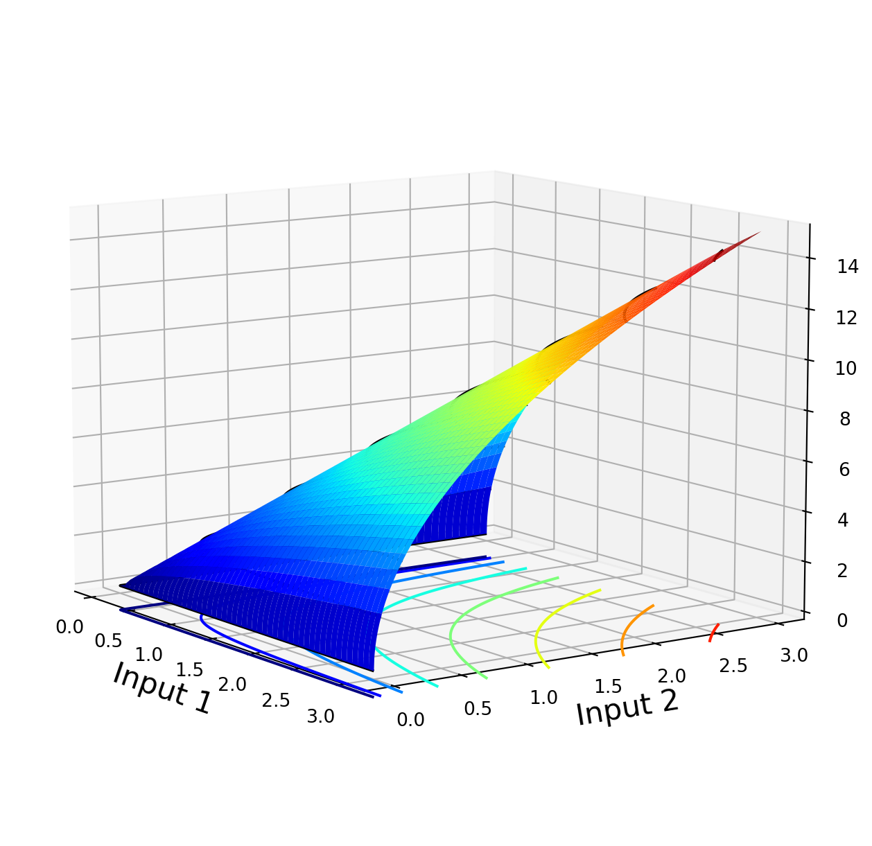
2.2 Exercise 2.2: Plotting a two-input production function surface

In this exercise, we plot the surface for a two-input Cobb-Douglas production function.

import matplotlib.cm as cm
import matplotlib.pyplot as plt
import numpy as np
from mpl_toolkits.mplot3d import Axes3D

def CobbDouglas(beta, X, Y):
    return 5 * X**beta * Y ** (1 - beta)

x = np.linspace(0, 3, 1000)
y = np.linspace(0, 3, 1000)
X, Y = np.meshgrid(x, y)
output = CobbDouglas(beta=0.5, X=X, Y=Y)

fig, ax = plt.subplots(figsize=(10, 8), subplot_kw={"projection": "3d"})
surf = ax.plot_surface(X, Y, output, cmap=cm.jet)
ax.contour(X, Y, output, 8, cmap=cm.jet, linestyles="solid", offset=-1)
ax.contour(X, Y, output, 8, colors="k", linestyles="solid")
ax.set_xlabel("Input 1", fontsize=16)
ax.set_ylabel("Input 2", fontsize=16)
ax.set_zlabel("Output", fontsize=16)
ax.view_init(10, -35)
plt.show()

# Remove all previous function and variable definitions before the next exercise
%reset

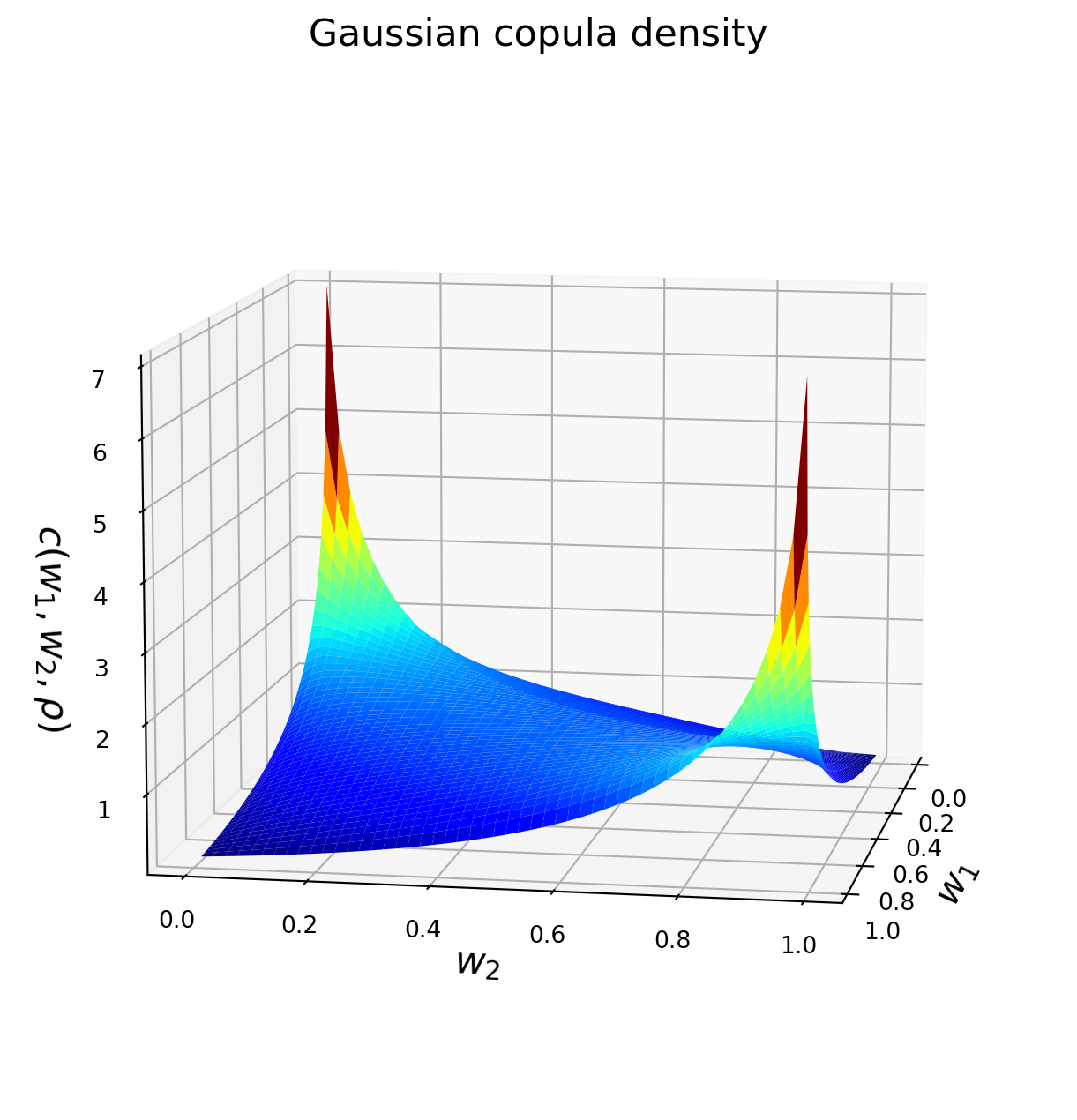
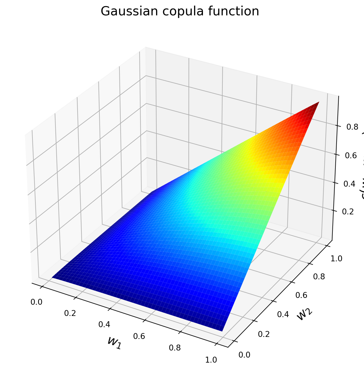
2.3 Exercise 2.3: Plotting a bivariate Gaussian Copula

In this exercise, we plot the bivariate Gaussian copula density and distribution function with $\rho = 0.5$.

import matplotlib.cm as cm
import matplotlib.pyplot as plt
import numpy as np
from mpl_toolkits.mplot3d import Axes3D
from scipy import stats

u1 = np.linspace(0.01, 0.99, 50)
u2 = np.linspace(0.01, 0.99, 50)
U1, U2 = np.meshgrid(u1, u2)
U = np.concatenate([U1.flatten().reshape(-1, 1), U2.flatten().reshape(-1, 1)], axis=1)

copula_pdf = stats.multivariate_normal.pdf(
    x=stats.norm.ppf(U), mean=np.zeros(2), cov=np.array([[1, 0.5], [0.5, 1]])
) / np.prod(stats.norm.pdf(stats.norm.ppf(U)), axis=1)
copula_cdf = stats.multivariate_normal.cdf(
    stats.norm.ppf(U), mean=np.zeros(2), cov=np.array([[1, 0.5], [0.5, 1]])
)

fig, ax = plt.subplots(figsize=(10, 8), subplot_kw={"projection": "3d"})
surf = ax.plot_surface(U1, U2, copula_pdf.reshape(50, 50), cmap=cm.jet)
ax.view_init(10, 10)
ax.set_xlabel(r"$w_{1}$", fontsize=16)
ax.set_ylabel(r"$w_{2}$", fontsize=16)
ax.set_zlabel(r"$c(w_{1}, w_{2}, \rho)$", fontsize=16)
ax.set_title(r"Gaussian copula density", fontsize = 16)
plt.show()

fig, ax = plt.subplots(figsize=(10, 8), subplot_kw={"projection": "3d"})
surf = ax.plot_surface(U1, U2, copula_cdf.reshape(50, 50), cmap=cm.jet)
ax.set_xlabel(r"$w_{1}$", fontsize=16)
ax.set_ylabel(r"$w_{2}$", fontsize=16)
ax.set_zlabel(r"$c(w_{1}, w_{2}, \rho)$", fontsize=16)
ax.set_title(r"Gaussian copula function", fontsize = 16)
plt.show()

# Remove all previous function and variable definitions before the next exercise
%reset

2.4 Exercise 2.4: Corrected Ordinary Least Squared (COLS) for deterministic frontier of the U.S. utilities data

In this exercise we implement a Corrected OLS (COLS) using a Cobb-Douglas production function.

The coefficient estimates suggest an increasing return to scale in electricity generation. The sign on labour ($\beta_{3}$) is surprising, but that coefficient is statistically insignificant.

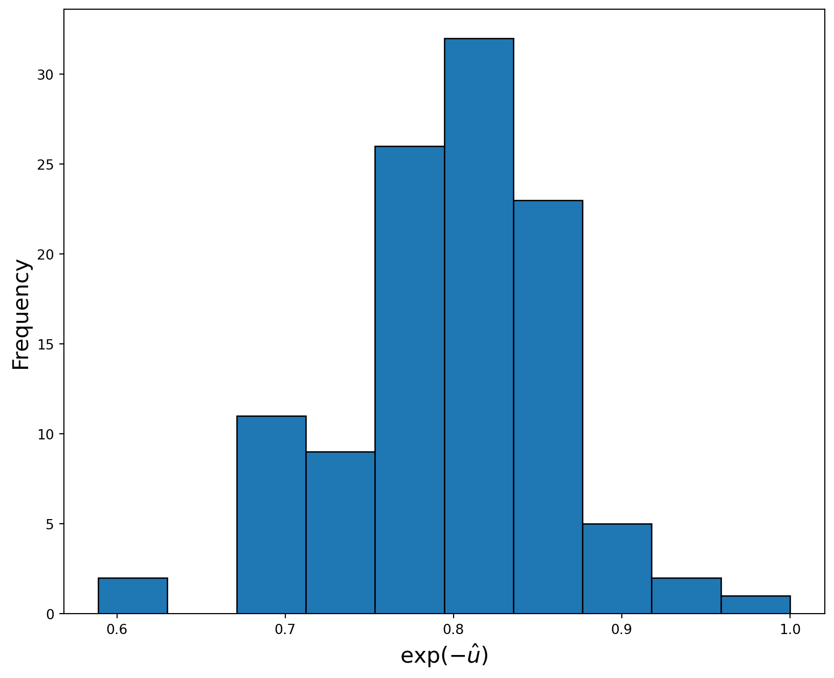
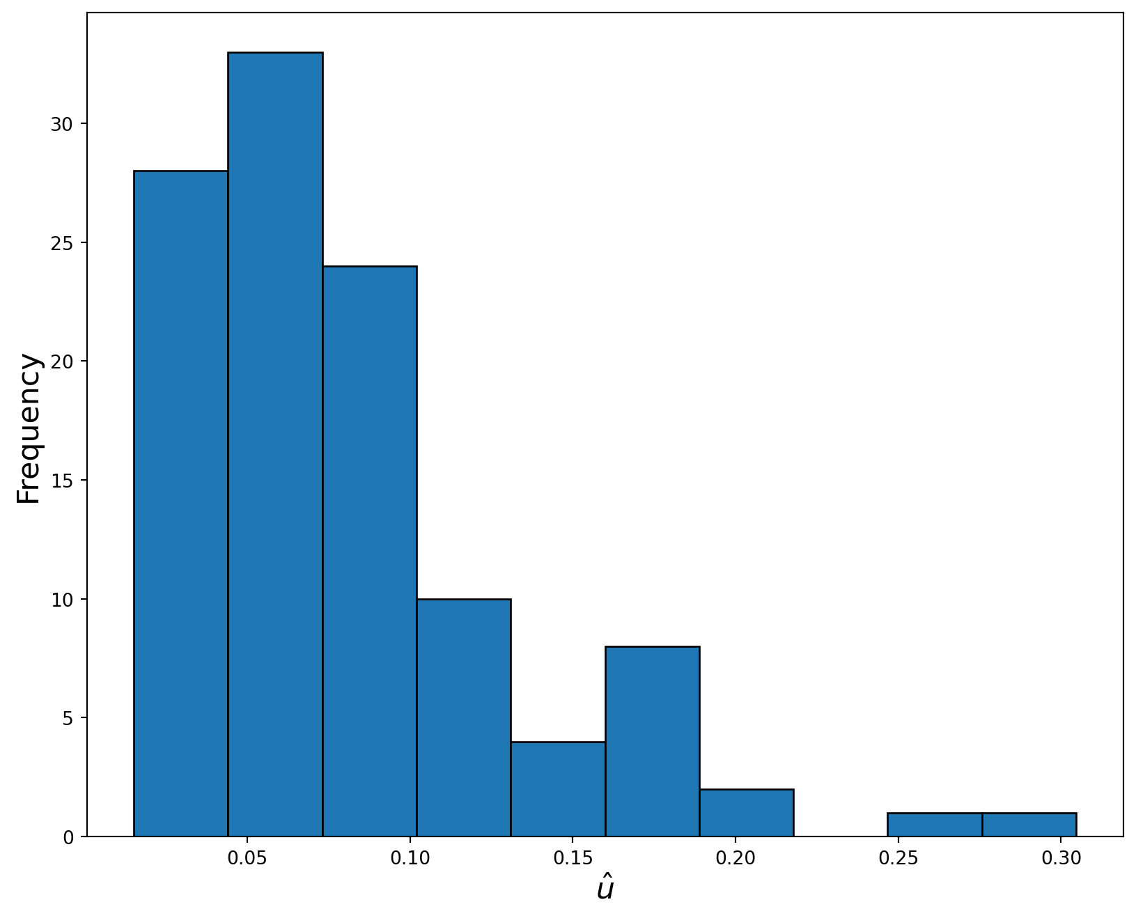
In order to obtain estimates of the inefficiencies, we generate the residuals and subtract their maximum from them. The result with a minus sign can be viewed as estimates of inefficiency $u_i$. Alternatively, if we calculate $\exp(-u_i)$, this will have the interpretation of production efficiency estimates, i.e. the percentage of potential electricity output actually produced by utility $i$. Figure plots the histogram of technical efficiency estimates from the COLS model. The distribution appears to be right skewed.

import matplotlib.pyplot as plt
import numpy as np
import pandas as pd
import statsmodels.formula.api as sm
from sklearn import linear_model

# Import data
production_data = pd.read_excel("cowing.xlsx")  # Inputs and outputs are in Logarithms

# Fit OLS model
colsd = sm.ols(
    formula="y ~ X1 + X2 + X3", data=production_data[["y", "X1", "X2", "X3"]]
)
colsd_fitted = colsd.fit()
print(colsd_fitted.summary())  

resids = colsd_fitted.resid  
u_star = -(resids - np.max(resids))  
eff_colsd = np.exp(-u_star)

# Plot a histogram of the technical efficiency estimates
figure = plt.figure(figsize=(10, 8))
plt.hist(eff_colsd, 10, edgecolor="k")
plt.xlabel("$\exp(-\hat{u})$", fontsize=16)
plt.ylabel("Frequency", fontsize=16)
plt.show()

                            OLS Regression Results                            
==============================================================================
Dep. Variable:                      y   R-squared:                       0.993
Model:                            OLS   Adj. R-squared:                  0.993
Method:                 Least Squares   F-statistic:                     5131.
Date:                Sun, 31 Mar 2024   Prob (F-statistic):          2.03e-115
Time:                        16:19:14   Log-Likelihood:                 120.15
No. Observations:                 111   AIC:                            -232.3
Df Residuals:                     107   BIC:                            -221.5
Df Model:                           3                                         
Covariance Type:            nonrobust                                         
==============================================================================
                 coef    std err          t      P>|t|      [0.025      0.975]
------------------------------------------------------------------------------
Intercept    -11.1657      0.205    -54.540      0.000     -11.572     -10.760
X1             0.0359      0.017      2.095      0.038       0.002       0.070
X2             1.0960      0.017     64.469      0.000       1.062       1.130
X3            -0.0210      0.023     -0.923      0.358      -0.066       0.024
==============================================================================
Omnibus:                       13.892   Durbin-Watson:                   1.602
Prob(Omnibus):                  0.001   Jarque-Bera (JB):               18.946
Skew:                          -0.638   Prob(JB):                     7.69e-05
Kurtosis:                       4.571   Cond. No.                         676.
==============================================================================

Notes:
[1] Standard Errors assume that the covariance matrix of the errors is correctly specified.

# Remove all previous function and variable definitions before the next exercise
%reset

2.5 Exercise 2.5: MLE for the US utilities data

In thi exercise, we perform Maximum Likelihood Estimation (MLE) for a Cobb-Douglas production function using a sample of 111 steam-electric power plants.

import matplotlib.pyplot as plt
import numpy as np
import pandas as pd
from scipy import stats
from scipy.optimize import minimize


def log_density(coefs, y, x1, x2, x3):

    [alpha, beta1, beta2, beta3, 
     sigma2u, sigma2v] = coefs[:]

    Lambda = np.sqrt(sigma2u / sigma2v)
    sigma2 = sigma2u + sigma2v
    sigma = np.sqrt(sigma2)

    # Composed errors from the production function equation
    eps = y - alpha - x1 * beta1 - x2 * beta2 - x3 * beta3

    # Compute the log density
    Den = (
        (2 / sigma)
        * stats.norm.pdf(eps / sigma)
        * stats.norm.cdf(-Lambda * eps / sigma)
    )
    logDen = np.log(Den)

    return logDen


def loglikelihood(coefs, y, x1, x2, x3):

    logDen = log_density(coefs, y, x1, x2, x3)
    log_likelihood = -np.sum(logDen)

    return log_likelihood


def estimate(y, x1, x2, x3):

    # Starting values for MLE
    alpha = -11
    beta1 = 0.03
    beta2 = 1.1
    beta3 = -0.01
    sigma2u = 0.01
    sigma2v = 0.0003

    theta0 = np.array([alpha, beta1, beta2, beta3, 
                       sigma2u, sigma2v])

    bounds = [(None, None) for x in range(len(theta0) - 2)] + [
        (1e-6, np.inf),
        (1e-6, np.inf),
    ]

    # Minimize the negative log-likelihood using numerical optimization.
    MLE_results = minimize(
        fun=loglikelihood,
        x0=theta0,
        method="L-BFGS-B",
        tol = 1e-6,
        options={"ftol": 1e-6, "maxiter": 1000, "maxfun": 6*1000},
        args=(y, x1, x2, x3),
        bounds=bounds,
    )

    theta = MLE_results.x  
    log_likelihood = MLE_results.fun  

    # Estimate standard errors
    delta = 1e-6
    grad = np.zeros((len(y), len(theta)))
    for i in range(len(theta)):
        theta1 = np.copy(theta)
        theta1[i] += delta
        grad[:, i] = (
            log_density(theta1, y, x1, x2, x3) - log_density(theta, y, x1, x2, x3)
        ) / delta

    OPG = grad.T @ grad  
    ster = np.sqrt(np.diag(np.linalg.inv(OPG)))

    return theta, ster, log_likelihood

# Import Data
production_data = pd.read_excel("cowing.xlsx")  # Inputs and outputs are in Logarithms
y = production_data["y"]  # Output
[x1, x2, x3] = [
    production_data["X1"],
    production_data["X2"],
    production_data["X3"],
]  

coefs, sterr, logMLE = estimate(y, x1, x2, x3)

Zscores = coefs / sterr
Pvalues = 2 * (1 - stats.norm.cdf(np.abs(Zscores)))
lower_ConfInt95 = stats.norm.ppf(0.025, loc=coefs, scale=sterr)
upper_ConfInt95 = stats.norm.ppf(0.975, loc=coefs, scale=sterr)

# Display the results as a table
results = pd.DataFrame(
    data={
        "Est": coefs,
        "StEr": sterr,
        "z-stat": Zscores,
        "p-val": Pvalues,
        "Lower 95% Conf Int": lower_ConfInt95,
        "Upper 95% Conf Int": upper_ConfInt95,
    },
    index=[
        r"$$\beta_{0}$$",
        r"$$\beta_{1}$$",
        r"$$\beta_{2}$$",
        r"$$\beta_{3}$$",
        r"$$\sigma^{2}_{u}$$",
        r"$$\sigma^{2}_{v}$$",
    ],
)
results = results.round(4)
display(results)
print(f"Log-likelihood: {round(logMLE, 4)}")

	Est	StEr	z-stat	p-val	Lower 95% Conf Int	Upper 95% Conf Int
$$\beta_{0}$$	-11.0003	0.1992	-55.2111	0.0000	-11.3908	-10.6097
$$\beta_{1}$$	0.0396	0.0191	2.0756	0.0379	0.0022	0.0770
$$\beta_{2}$$	1.0867	0.0203	53.6057	0.0000	1.0470	1.1265
$$\beta_{3}$$	-0.0207	0.0257	-0.8058	0.4204	-0.0711	0.0297
$$\sigma^{2}_{u}$$	0.0107	0.0033	3.2188	0.0013	0.0042	0.0172
$$\sigma^{2}_{v}$$	0.0027	0.0009	3.1740	0.0015	0.0010	0.0044

Log-likelihood: -123.0568

2.5.1 Prediction of Technical Inefficiencies, $\hat{u}_{i}$

[
    estimated_alpha,
    estimated_beta1,
    estimated_beta2,
    estimated_beta3,
    estimated_sigma2u,
    estimated_sigma2v,
] = coefs[:6]

# Composed errors from the production function equation
eps = (
    y
    - estimated_alpha
    - x1 * estimated_beta1
    - x2 * estimated_beta2
    - x3 * estimated_beta3
)

sigma = np.sqrt(estimated_sigma2u + estimated_sigma2v)
lam = np.sqrt(coefs[4] / estimated_sigma2v)

bi = (eps * lam) / sigma
hazard = stats.norm.pdf(bi) / (1 - stats.norm.cdf(bi))
sigstar = np.sqrt(estimated_sigma2u * estimated_sigma2v) / sigma

Eu = sigstar * (hazard - bi)  # Technical inefficiency estimates
Vu = (sigstar**2) * (
    1 + bi * hazard - hazard * hazard
)  # Variance of technical inefficiency

figure = plt.figure(figsize=(10, 8))
plt.hist(Eu, edgecolor="k", bins=10)
plt.xlabel("$\hat{u}$", fontsize=16)
plt.ylabel("Frequency", fontsize=16)
plt.show()

# Remove all previous function and variable definitions before the next exercise
%reset

2.6 Exercise 2.6: MLE for models with heteroskedasticity

In this exercise we perform Maximum Likelihood Estimation for a Cobb-Douglas production function with heteroskedasticity (non-constant variance) in $u$, that is $\sigma^{2}_{ui}=\exp(\mathbf{z}_{i}'\omega_u)$, for 196 dairy farms. The output is the log amount of milk production and the inputs are labor hours (llabor), feed (lfeed), the number of cows (lcattle) and the land size of the farm (lland) all in logarithms. The environmental variable comp is IT expenditure as a percentage of total expenditure.

import numpy as np
import pandas as pd
from scipy import stats
from scipy.optimize import minimize


def log_density(coefs, y, x1, x2, x3, x4, z1):
    # Get parameters
    [alpha, beta1, beta2, beta3, beta4, 
     omega0, omega1, sigma2v] = coefs[:]

    sigma2u = np.exp(omega0 + omega1 * z1)  # Heteroskedastic sigma2u
    Lambda = np.sqrt(sigma2u / sigma2v)
    sigma2 = sigma2u + sigma2v
    sigma = np.sqrt(sigma2)

    # Composed errors from the production function equation
    eps = y - alpha - x1 * beta1 - x2 * beta2 - x3 * beta3 - x4 * beta4

    # Compute log-density
    Den = (
        2 / sigma * stats.norm.pdf(eps / sigma) * stats.norm.cdf(-Lambda * eps / sigma)
    )
    Den = np.where(
        np.abs(Den) < 1e-5, 1e-5, Den
    )  # Adjust small densities for numerical precision
    logDen = np.log(Den)

    return logDen


def loglikelihood(coefs, y, x1, x2, x3, x4, z1):
    # Obtain the log likelihood
    logDen = log_density(coefs, y, x1, x2, x3, x4, z1)
    log_likelihood = -np.sum(logDen)

    return log_likelihood


def estimate(y, x1, x2, x3, x4, z1):
    """
    Estimate model parameters by maximizing the log-likelihood function and compute standard errors.
    """

    # Starting values for MLE
    alpha = 7.7
    beta1 = 0.1
    beta2 = 0.15
    beta3 = 0.75
    beta4 = 0.03
    omega0 = -3
    omega1 = -0.015  # Coefficient for z1
    sigma2v = 0.005

    # Initial parameter vector
    theta0 = np.array([alpha, beta1, beta2, beta3, beta4, 
                       omega0, omega1, sigma2v])

    bounds = [(None, None) for x in range(len(theta0) - 1)] + [(1e-6, np.inf)]

    # Minimize the negative log-likelihood using numerical optimization.
    MLE_results = minimize(
        fun=loglikelihood,
        x0=theta0,
        method="L-BFGS-B",
        tol = 1e-6,
        options={"ftol": 1e-6, "maxiter": 1000, "maxfun": 6*1000, "maxcor": 500},
        args=(y, x1, x2, x3, x4, z1)
    )

    theta = MLE_results.x 
    log_likelihood = MLE_results.fun * -1

    # Estimate standard errors
    delta = 1e-6
    grad = np.zeros((len(y), len(theta)))
    for i in range(len(theta)):
        theta1 = np.copy(theta)
        theta1[i] += delta
        grad[:, i] = (
            log_density(theta1, y, x1, x2, x3, x4, z1)
            - log_density(theta, y, x1, x2, x3, x4, z1)
        ) / delta

    OPG = grad.T @ grad  # Outer product of gradient
    ster = np.sqrt(np.diag(np.linalg.inv(OPG)))

    return theta, ster, log_likelihood

# Import data
production_data = pd.read_csv("dairy.csv")  # Inputs and outputs are in Logarithms
y = production_data["ly"].values
[x1, x2, x3, x4] = [
    production_data["llabor"].values,
    production_data["lfeed"].values,
    production_data["lcattle"].values,
    production_data["lland"].values,
]
# Environmental variable
z1 = production_data["comp"]

# Estimate coefficients via MLE and standard errors for SFA model
coefs, sterr, logMLE = estimate(y, x1, x2, x3, x4, z1)

Zscores = coefs / sterr
Pvalues = 2 * (1 - stats.norm.cdf(np.abs(Zscores)))
lower_ConfInt95 = stats.norm.ppf(0.025, loc=coefs, scale=sterr)
upper_ConfInt95 = stats.norm.ppf(0.975, loc=coefs, scale=sterr)

# Display the results as a table
results = pd.DataFrame(
    columns=["Est", "StEr", "z-stat", "p-val", "[95%Conf.", "Interv]"],
    index=[
        r"$$\alpha$$",
        "llabor",
        "lfeed",
        "lcattle",
        "lland",
        " ",
        r"$$\omega_{0}$$",
        "comp",
        r"$$\sigma^{2}_{v}$$",
    ],
)

coefs = np.round(coefs.reshape(-1, 1), 3)
sterr = np.round(sterr.reshape(-1, 1), 3)
Zscores = np.round(Zscores.reshape(-1, 1), 3)
Pvalues = np.round(Pvalues.reshape(-1, 1), 3)
lower_ConfInt95 = np.round(lower_ConfInt95.reshape(-1, 1), 3)
upper_ConfInt95 = np.round(upper_ConfInt95.reshape(-1, 1), 3)

# Get the production frontier parameter estimates, standard errors and confidence intervals
frontier = np.concatenate(
    [
        coefs[:5],
        sterr[:5],
        Zscores[:5],
        Pvalues[:5],
        lower_ConfInt95[:5],
        upper_ConfInt95[:5],
    ],
    axis=1,
)

# Get the parameters for the heteroskedastic technical inefficiency parameterization
Omegas = np.concatenate(
    [
        coefs[5:7],
        sterr[5:7],
        Zscores[5:7],
        Pvalues[5:7],
        lower_ConfInt95[5:7],
        upper_ConfInt95[5:7],
    ],
    axis=1,
)

sigmas = np.array(
    [coefs[7], sterr[7], Zscores[7], Pvalues[7], lower_ConfInt95[7], upper_ConfInt95[7]]
).T

print("\nLog-Likelihood", round(logMLE, 3))
results.iloc[0:5, :] = frontier
results.iloc[5, :] = np.full(shape=(1, 6), fill_value=" ")
results.iloc[6:8, :] = Omegas
results.iloc[8:, :] = sigmas
display(results)


Log-Likelihood 110.545

	Est	StEr	z-stat	p-val	[95%Conf.	Interv]
$$\alpha$$	7.701	0.493	15.617	0.0	6.734	8.667
llabor	0.105	0.046	2.282	0.023	0.015	0.196
lfeed	0.158	0.04	3.992	0.0	0.08	0.235
lcattle	0.752	0.064	11.703	0.0	0.626	0.878
lland	0.034	0.042	0.79	0.43	-0.05	0.117

$$\omega_{0}$$	-3.0	0.532	-5.636	0.0	-4.043	-1.957
comp	-0.016	0.094	-0.17	0.865	-0.2	0.168
$$\sigma^{2}_{v}$$	0.005	0.002	1.894	0.058	-0.0	0.009

# Remove all previous function and variable definitions before the next exercise
%reset

2.7 Exercise 2.7: MLE of truncated normal distribution with $\mu \neq 0$

This exercise estimates a Cobb-Douglas production function with a truncated normal distribution for technical inefficiency with non-zero (constant) mean ($\mu \neq 0)$ via maximum likelihood using the the dairy farm production data.

import matplotlib.pyplot as plt
import numdifftools as nd
import numpy as np
import pandas as pd
from scipy import stats
from scipy.optimize import minimize


def log_density(coefs, y, x1, x2, x3, x4):
    # Get parameters
    [alpha, beta1, beta2, beta3, beta4, 
     mu, sigma2u, sigma2v] = coefs[:]

    # Composed errors from the production function equation
    eps = y - alpha - x1 * beta1 - x2 * beta2 - x3 * beta3 - x4 * beta4
    sigma2 = sigma2u + sigma2v
    mu_star = (sigma2v * mu - sigma2u * eps) / sigma2
    sigma2_star = (sigma2u * sigma2v) / sigma2

    Den = stats.norm.pdf((eps + mu) / np.sqrt(sigma2)) / (
        np.sqrt(sigma2)
        * (
            stats.norm.cdf(mu / np.sqrt(sigma2u))
            / stats.norm.cdf(mu_star / np.sqrt(sigma2_star))
        )
    )
    Den = np.where(
        np.abs(Den) < 1e-5, 1e-5, Den
    )  # Adjust small densities for numerical precision
    logDen = np.log(Den)

    return logDen


def loglikelihood(coefs, y, x1, x2, x3, x4):
    # Obtain the log likelihood
    logDen = log_density(coefs, y, x1, x2, x3, x4)
    log_likelihood = -np.sum(logDen)

    return log_likelihood


def estimate(y, x1, x2, x3, x4):
    """
    Estimate model parameters by maximizing the log-likelihood function and compute standard errors.
    """

    # Starting values for MLE
    alpha = 7.7
    beta1 = 0.1
    beta2 = 0.15
    beta3 = 0.7
    beta4 = 0.03
    sigma2u = 0.17
    sigma2v = 0.005
    mu = -1.2

    # Initial parameter vector
    theta0 = np.array([alpha, beta1, beta2, beta3, beta4, 
                       mu, sigma2u, sigma2v])

    # Bounds to ensure sigma2v and sigma2u are positive
    bounds = [(None, None) for x in range(len(theta0) - 2)] + [
        (1e-6, np.inf),
        (1e-6, np.inf),
    ]

    # Minimize the negative log-likelihood using numerical optimization.
    MLE_results = minimize(
        fun=loglikelihood,
        x0=theta0,
        method="L-BFGS-B",
        tol = 1e-6,
        options={"ftol": 1e-6, "maxiter": 1000, "maxfun": 6*1000, "maxcor": 500},
        args=(y, x1, x2, x3, x4),
        bounds=bounds,
    )

    theta = MLE_results.x  # Estimated parameter vector
    logMLE = MLE_results.fun * -1  # Log-likelihood at the solution

    # Estimate standard errors
    # Inverse of the Hessian approach
    hessian = nd.Hessian(f=loglikelihood, method="central", step=1e-5)
    ster = np.sqrt(np.diag(np.linalg.inv(hessian(theta, y, x1, x2, x3, x4))))

    return theta, ster, logMLE

# Import data
production_data = pd.read_csv("dairy.csv")  # Inputs and outputs are in Logarithms
y = production_data["ly"].values
[x1, x2, x3, x4] = [
    production_data["llabor"].values,
    production_data["lfeed"].values,
    production_data["lcattle"].values,
    production_data["lland"].values,
]

# Estimate coefficients via MLE and standard errors for SFA model
coefs, sterr, logMLE = estimate(y, x1, x2, x3, x4)

Zscores = coefs / sterr
Pvalues = 2 * (1 - stats.norm.cdf(np.abs(Zscores)))
lower_ConfInt95 = stats.norm.ppf(0.025, loc=coefs, scale=sterr)
upper_ConfInt95 = stats.norm.ppf(0.975, loc=coefs, scale=sterr)

# Display the results as a table
results = pd.DataFrame(
    columns=["Est", "StEr", "z-stat", "p-val", "[95%Conf.", "Interv]"],
    index=[
        r"$$\alpha$$",
        "llabor",
        "lfeed",
        "lcattle",
        "lland",
        " ",
        r"$$\mu$$",
        r"$$\sigma^{2}_{u}$$",
        r"$$\sigma^{2}_{v}$$",
    ],
)

coefs = np.round(coefs.reshape(-1, 1), 3)
sterr = np.round(sterr.reshape(-1, 1), 3)
Zscores = np.round(Zscores.reshape(-1, 1), 3)
Pvalues = np.round(Pvalues.reshape(-1, 1), 3)
lower_ConfInt95 = np.round(lower_ConfInt95.reshape(-1, 1), 3)
upper_ConfInt95 = np.round(upper_ConfInt95.reshape(-1, 1), 3)

# Get production function parameter estimates
frontier = np.concatenate(
    [
        coefs[:5],
        sterr[:5],
        Zscores[:5],
        Pvalues[:5],
        lower_ConfInt95[:5],
        upper_ConfInt95[:5],
    ],
    axis=1,
)

# Get sigma2u and sigma2v parameters
mu = np.array(
    [coefs[5], sterr[5], Zscores[5], Pvalues[5], lower_ConfInt95[5], upper_ConfInt95[5]]
).T
sigmas = np.concatenate(
    [
        coefs[6:],
        sterr[6:],
        Zscores[6:],
        Pvalues[6:],
        lower_ConfInt95[6:],
        upper_ConfInt95[6:],
    ],
    axis=1,
)

print("\nLog-Likelihood", round(logMLE, 3))
results.iloc[0:5, :] = frontier
results.iloc[5, :] = np.full(shape=(1, 6), fill_value=" ")
results.iloc[6, :] = mu
results.iloc[7:, :] = sigmas
display(results)


Log-Likelihood 110.843

/var/folders/q0/9kb46g7n1_57dfk7vtdsv8t4w169ch/T/ipykernel_41229/339382716.py:23: RuntimeWarning: divide by zero encountered in divide
  stats.norm.cdf(mu / np.sqrt(sigma2u))

	Est	StEr	z-stat	p-val	[95%Conf.	Interv]
$$\alpha$$	7.697	0.49	15.708	0.0	6.737	8.657
llabor	0.101	0.044	2.327	0.02	0.016	0.187
lfeed	0.152	0.038	4.013	0.0	0.078	0.227
lcattle	0.751	0.058	13.006	0.0	0.638	0.865
lland	0.044	0.039	1.116	0.265	-0.033	0.121

$$\mu$$	-1.2	4.387	-0.273	0.784	-9.799	7.399
$$\sigma^{2}_{u}$$	0.173	0.491	0.353	0.724	-0.789	1.136
$$\sigma^{2}_{v}$$	0.008	0.003	2.829	0.005	0.002	0.013

# Remove all previous function and variable definitions before the next exercise
%reset

2.8 Exercise 2.8: MLE of truncated normal with $\mu_{i} = z_{i}^{\prime}\delta$ and $\sigma^{2}_{ui} = e^{({z_{i}^{\prime}\omega})}$

This exercise estimates a Cobb-Douglas production function using a truncated normal distribution for technical inefficiency via maximum likelihood for 196 dairy farms. Marginal effects are also computed.

import numdifftools as nd
import numpy as np
import pandas as pd
from scipy import stats
from scipy.optimize import minimize


def log_density(coefs, y, x1, x2, x3, x4, z1):
    
    # get parameters
    [alpha,beta1,beta2,beta3,beta4,
     gamma0,gamma1,omega0,omega1,sigma2v,] = coefs[:10]

    mu = gamma0 + gamma1 * z1
    sigma2u = np.exp(omega0 + omega1 * z1)
    # Composed errors from the production function equation
    eps = y - alpha - x1 * beta1 - x2 * beta2 - x3 * beta3 - x4 * beta4
    sigma2 = sigma2u + sigma2v
    mu_star = (sigma2v * mu - sigma2u * eps) / sigma2
    sigma2_star = (sigma2u * sigma2v) / sigma2

    Den = stats.norm.pdf((eps + mu) / np.sqrt(sigma2)) / (
        np.sqrt(sigma2)
        * (
            stats.norm.cdf(mu / np.sqrt(sigma2u))
            / stats.norm.cdf(mu_star / np.sqrt(sigma2_star))
        )
    )
    Den = np.where(
        np.abs(Den) < 1e-6, 1e-6, Den
    )  # Adjust small densities for numerical precision
    logDen = np.log(Den)

    return logDen


def loglikelihood(coefs, y, x1, x2, x3, x4, z1):
    # Obtain the log likelihood
    logDen = log_density(coefs, y, x1, x2, x3, x4, z1)
    log_likelihood = -np.sum(logDen)

    return log_likelihood


def estimate(y, x1, x2, x3, x4, z1):
    """
    Estimate model parameters by maximizing the log-likelihood function and compute standard errors.
    """

    # Starting values for MLE
    alpha = 7.5
    beta1 = 0.1
    beta2 = 0.15
    beta3 = 0.7
    beta4 = 0.03
    gamma0 = 7
    gamma1 = -1.5  # Coefficient for z1 in non-constant mu equation
    omega0 = -3
    omega1 = 0.3  # Coefficient for z1 in non-constant variance equation
    sigma2v = 0.008

    # Initial parameter vector
    theta0 = np.array(
        [alpha, beta1, beta2, beta3, beta4, gamma0, gamma1, omega0, omega1, sigma2v]
    )

    # Bounds to ensure sigma2v and sigma2u are positive
    bounds = [(None, None) for x in range(len(theta0) - 1)] + [(1e-6, np.inf)]

    MLE_results = minimize(
        loglikelihood,
        theta0,
        method="L-BFGS-B",
        tol = 1e-6,
        options={"ftol": 1e-6, "maxiter": 1000, "maxfun": 6*1000, "maxcor": 500},
        args=(y, x1, x2, x3, x4, z1),
        bounds=bounds,
    )

    theta = MLE_results.x
    logMLE = MLE_results.fun * -1

    # Standard errors
    # Inverse of the Hessian approach
    hessian = nd.Hessian(f=loglikelihood, method="central", step=1e-6)
    ster = np.sqrt(np.diag(np.linalg.inv(hessian(theta, y, x1, x2, x3, x4, z1))))
    return theta, ster, logMLE

production_data = pd.read_csv("dairy.csv")  # Inputs and outputs are in Logarithms
# output
y = production_data["ly"]
# Inputs
x1 = production_data["llabor"]
x2 = production_data["lfeed"]
x3 = production_data["lcattle"]
x4 = production_data["lland"]
# Environmental variable
z1 = production_data["comp"]

# Estimate coefficients via MLE and standard errors for SFA model
coefs, sterr, logMLE = estimate(y, x1, x2, x3, x4, z1)
Zscores = coefs / sterr
Pvalues = 2 * (1 - stats.norm.cdf(np.abs(Zscores)))
lower_ConfInt95 = stats.norm.ppf(0.025, loc=coefs, scale=sterr)
upper_ConfInt95 = stats.norm.ppf(0.975, loc=coefs, scale=sterr)

# Display the results as a table
results = pd.DataFrame(
    columns=["Est", "StEr", "z-stat", "p-val", "[95%Conf.", "Interv]"],
    index=[
        r"$$\alpha$$",
        "llabor",
        "lfeed",
        "lcattle",
        "lland",
        " ",
        r"$$\delta_{0}$$",
        r"$$\delta_{1}$$",
        r"$$\omega_{0}$$",
        r"$$\omega_{1}$$",
        r"$$\sigma^{2}_{v}$$",
    ],
)

coefs = np.round(coefs.reshape(-1, 1), 3)
sterr = np.round(sterr.reshape(-1, 1), 3)
Zscores = np.round(Zscores.reshape(-1, 1), 3)
Pvalues = np.round(Pvalues.reshape(-1, 1), 3)
lower_ConfInt95 = np.round(lower_ConfInt95.reshape(-1, 1), 3)
upper_ConfInt95 = np.round(upper_ConfInt95.reshape(-1, 1), 3)

frontier = np.concatenate(
    [
        coefs[:5],
        sterr[:5],
        Zscores[:5],
        Pvalues[:5],
        lower_ConfInt95[:5],
        upper_ConfInt95[:5],
    ],
    axis=1,
)

mu = np.concatenate(
    [
        coefs[5:7],
        sterr[5:7],
        Zscores[5:7],
        Pvalues[5:7],
        lower_ConfInt95[5:7],
        upper_ConfInt95[5:7],
    ],
    axis=1,
)
usigma = np.concatenate(
    [
        coefs[7:9],
        sterr[7:9],
        Zscores[7:9],
        Pvalues[7:9],
        lower_ConfInt95[7:9],
        upper_ConfInt95[7:9],
    ],
    axis=1,
)
vsigma = np.array(
    [coefs[9], sterr[9], Zscores[9], Pvalues[9], lower_ConfInt95[9], upper_ConfInt95[9]]
).T

print("\nLog-Likelihood", round(logMLE, 3))
results.iloc[0:5, :] = frontier
results.iloc[5, :] = np.full(shape=(1, 6), fill_value=" ")
results.iloc[6:8, :] = mu
results.iloc[8:10, :] = usigma
results.iloc[10, :] = vsigma
display(results)

/var/folders/q0/9kb46g7n1_57dfk7vtdsv8t4w169ch/T/ipykernel_41229/2332912828.py:25: RuntimeWarning: divide by zero encountered in divide
  stats.norm.cdf(mu / np.sqrt(sigma2u))


Log-Likelihood 118.325

	Est	StEr	z-stat	p-val	[95%Conf.	Interv]
$$\alpha$$	7.751	0.476	16.296	0.0	6.819	8.684
llabor	0.101	0.042	2.389	0.017	0.018	0.184
lfeed	0.145	0.037	3.948	0.0	0.073	0.218
lcattle	0.741	0.056	13.133	0.0	0.631	0.852
lland	0.053	0.038	1.41	0.159	-0.021	0.127

$$\delta_{0}$$	7.1	5.199	1.366	0.172	-3.09	17.289
$$\delta_{1}$$	-1.579	1.228	-1.286	0.198	-3.985	0.828
$$\omega_{0}$$	-3.654	1.04	-3.514	0.0	-5.692	-1.616
$$\omega_{1}$$	0.372	0.066	5.635	0.0	0.243	0.501
$$\sigma^{2}_{v}$$	0.008	0.002	4.717	0.0	0.005	0.012

2.8.1 Estimate Marginal Effects

# Marginal effect of comp on E(u)
exogenous_data = np.column_stack([np.ones(len(z1)), z1])
mu_vector = exogenous_data @ coefs[5:7]
sigma_vector = np.sqrt(np.exp(exogenous_data @ coefs[7:9]))
Lambda = mu_vector / sigma_vector
cdf = stats.norm.cdf(Lambda)
pdf = stats.norm.pdf(Lambda)
ratio = pdf / cdf

marginal_effects_Eu = coefs[6] * (1 - Lambda * ratio - (ratio**2)) + coefs[8] * (
    sigma_vector / 2
) * ((1 + (Lambda**2)) * ratio + (Lambda * ratio**2))
average_marginal_effect_Eu = round(np.mean(marginal_effects_Eu), 5)
print(
    f'The average marginal effect of the variable "comp" on the unconditional E(u) is {average_marginal_effect_Eu}'
)

The average marginal effect of the variable "comp" on the unconditional E(u) is -0.03591

# Remove all previous function and variable definitions before the next exercise
%reset

2.9 Exercise 2.9: An SF model with the scaling property

This exercise estimates a Cobb-Douglas production function using a truncated normal distribution with the scaling property for technical inefficiency via maximum likelihood for 196 dairy farms.

import numdifftools as nd
import numpy as np
import pandas as pd
from scipy import stats
from scipy.optimize import minimize


def log_density(coefs, y, x1, x2, x3, x4, z1):
    
    # get parameters
    [alpha, beta1, beta2, beta3, beta4, 
     gamma1, tau, cu, sigma2v] = coefs[:9]

    # Composed errors from the production function equation
    eps = y - alpha - x1 * beta1 - x2 * beta2 - x3 * beta3 - x4 * beta4

    sigma2u_tilde = cu * np.exp(2 * (gamma1 * z1))
    u_tilde = tau * np.exp(gamma1 * z1)
    sigma2 = sigma2v + sigma2u_tilde
    u_star = (sigma2v * u_tilde - sigma2u_tilde * eps) / sigma2
    sigma2_star = (sigma2v * sigma2u_tilde) / sigma2

    Den = stats.norm.pdf((eps + u_tilde) / np.sqrt(sigma2)) / (
        np.sqrt(sigma2)
        * (
            stats.norm.cdf(u_tilde / np.sqrt(sigma2u_tilde))
            / stats.norm.cdf(u_star / np.sqrt(sigma2_star))
        )
    )
    Den = np.where(
        np.abs(Den) < 1e-5, 1e-5, Den
    )  # Adjust small densities for numerical precision
    logDen = np.log(Den)  # Log density

    return logDen


def loglikelihood(coefs, y, x1, x2, x3, x4, z1):
    # Obtain the log likelihood
    logDen = log_density(coefs, y, x1, x2, x3, x4, z1)
    log_likelihood = -np.sum(logDen)

    return log_likelihood


def estimate(y, x1, x2, x3, x4, z1):
    
    # Starting values for MLE
    alpha = 7.7
    beta1 = 0.1
    beta2 = 0.15
    beta3 = 0.7
    beta4 = 0.03
    gamma1 = (-0.008)  # Coefficient for z1 in the scaling function h(.). No constant is included in the gamma parameter vector
    tau = -1  # Mean of half-normal distribution common to all observations
    cu = 0.15  # Variance of half-normal distribution common to all observations
    sigma2v = 0.008

    # Initial parameter vector
    theta0 = [alpha, beta1, beta2, beta3, beta4, 
              gamma1, tau, cu, sigma2v]

    bounds = [(None, None) for x in range(len(theta0) - 2)] + [
        (1e-6, np.inf),
        (1e-6, np.inf),
    ]

    MLE_results = minimize(
        loglikelihood,
        theta0,
        method="L-BFGS-B",
        tol = 1e-6,
        options={"ftol": 1e-6, "maxiter": 1000, "maxfun": 6*1000, "maxcor": 500},
        args=(y, x1, x2, x3, x4, z1),
        bounds=bounds,
    )

    theta = MLE_results.x
    logMLE = MLE_results.fun * -1

    # Standard errors
    # Inverse of the Hessian approach
    hessian = nd.Hessian(f=loglikelihood, method="central", step=1e-6)
    ster = np.sqrt(np.diag(np.linalg.inv(hessian(theta, y, x1, x2, x3, x4, z1))))

    return theta, ster, logMLE

production_data = pd.read_csv("dairy.csv")  # Inputs and outputs are in Logarithms
# Output
y = production_data["ly"]
# Inputs
x1 = production_data["llabor"]
x2 = production_data["lfeed"]
x3 = production_data["lcattle"]
x4 = production_data["lland"]
# Environmental variable
z1 = production_data["comp"]

# Estimate coefficients via MLE and standard errors for SFA model
coefs, sterr, logMLE = estimate(y, x1, x2, x3, x4, z1)

Zscores = coefs / sterr
Pvalues = 2 * (1 - stats.norm.cdf(np.abs(Zscores)))
lower_ConfInt95 = stats.norm.ppf(0.025, loc=coefs, scale=sterr)
upper_ConfInt95 = stats.norm.ppf(0.975, loc=coefs, scale=sterr)

# Display the results as a table
results = pd.DataFrame(
    columns=["Est", "StEr", "z-stat", "p-val", "[95%Conf.", "Interv]"],
    index=[
        r"$$\alpha$$",
        "llabor",
        "lfeed",
        "lcattle",
        "lland",
        " ",
        "hscale",
        r"$$\tau$$",
        "Cu",
        r"$$\sigma^{2}_{v}$$",
    ],
)

coefs = np.round(coefs.reshape(-1, 1), 3)
sterr = np.round(sterr.reshape(-1, 1), 3)
Zscores = np.round(Zscores.reshape(-1, 1), 3)
Pvalues = np.round(Pvalues.reshape(-1, 1), 3)
lower_ConfInt95 = np.round(lower_ConfInt95.reshape(-1, 1), 3)
upper_ConfInt95 = np.round(upper_ConfInt95.reshape(-1, 1), 3)

frontier = np.concatenate(
    [
        coefs[:5],
        sterr[:5],
        Zscores[:5],
        Pvalues[:5],
        lower_ConfInt95[:5],
        upper_ConfInt95[:5],
    ],
    axis=1,
)

scaling_ceofs = np.concatenate(
    [
        coefs[5:8],
        sterr[5:8],
        Zscores[5:8],
        Pvalues[5:8],
        lower_ConfInt95[5:8],
        upper_ConfInt95[5:8],
    ],
    axis=1,
)
vsigma = np.array(
    [coefs[8], sterr[8], Zscores[8], Pvalues[8], lower_ConfInt95[8], upper_ConfInt95[8]]
).T

print("\nLog-Likelihood", round(logMLE, 3))
results.iloc[0:5, :] = frontier
results.iloc[5, :] = np.full(shape=(1, 6), fill_value=" ")
results.iloc[6:9, :] = scaling_ceofs
results.iloc[9, :] = vsigma
display(results)

/var/folders/q0/9kb46g7n1_57dfk7vtdsv8t4w169ch/T/ipykernel_41229/2857292431.py:26: RuntimeWarning: divide by zero encountered in divide
  stats.norm.cdf(u_tilde / np.sqrt(sigma2u_tilde))


Log-Likelihood 110.859

	Est	StEr	z-stat	p-val	[95%Conf.	Interv]
$$\alpha$$	7.697	0.491	15.674	0.0	6.735	8.66
llabor	0.101	0.044	2.316	0.021	0.016	0.187
lfeed	0.153	0.038	4.019	0.0	0.078	0.228
lcattle	0.752	0.058	12.965	0.0	0.639	0.866
lland	0.043	0.039	1.08	0.28	-0.035	0.12

hscale	-0.007	0.047	-0.143	0.886	-0.099	0.085
$$\tau$$	-0.999	3.241	-0.308	0.758	-7.351	5.352
Cu	0.158	0.364	0.435	0.664	-0.554	0.871
$$\sigma^{2}_{v}$$	0.008	0.003	2.796	0.005	0.002	0.013

# Remove all previous function and variable definitions before the next exercise
%reset

2.10 Exercise 2.10: An SF model with an exponential distribution for $\mu_{i}$

This exercise estimates a Cobb-Douglas production function with an exponential distribution for technical inefficiency via maximum likelihood for 196 dairy farms. To account for heteroskedasticity, the exponential distribution parameter is $\eta^{2} = e^{({z}_{i}^{\prime}{\delta})}$.

import numdifftools as nd
import numpy as np
import pandas as pd
from scipy import stats
from scipy.optimize import minimize


def log_density(coefs, y, x1, x2, x3, x4, z1):
    # Get parameters
    [alpha, beta1, beta2, beta3, beta4, 
     omega0, omega1, sigma2v] = coefs[:9]

    nu2 = np.exp(omega0 + omega1 * z1)

    # Composed errors from the production function equation
    eps = y - alpha - x1 * beta1 - x2 * beta2 - x3 * beta3 - x4 * beta4

    cdf_term = stats.norm.cdf(
        (-eps / np.sqrt(sigma2v)) - (np.sqrt(sigma2v) / np.sqrt(nu2))
    )
    Den = (
        1
        / np.sqrt(nu2)
        * np.exp((eps / np.sqrt(nu2)) + (sigma2v / (2 * nu2)))
        * cdf_term
    )
    logDen = np.log(Den)

    return logDen


def loglikelihood(coefs, y, x1, x2, x3, x4, z1):
    
    # Obtain the log likelihood
    logDen = log_density(coefs, y, x1, x2, x3, x4, z1)
    log_likelihood = -np.sum(logDen)

    return log_likelihood


def estimate(y, x1, x2, x3, x4, z1):
    # Starting values for MLE
    alpha = 7.5
    beta1 = 0.1
    beta2 = 0.15
    beta3 = 0.7
    beta4 = 0.03
    omega0 = -4
    omega1 = -0.005  # Coefficient for z1
    sigma2v = 0.01

    # Initial parameter vector
    theta0 = [alpha, beta1, beta2, beta3, beta4, omega0, omega1, sigma2v]

    # Bounds to ensure sigma2v and sigma2u are > 0
    bounds = [(None, None) for x in range(len(theta0) - 1)] + [(1e-4, np.inf)]

    MLE_results = minimize(
        loglikelihood,
        theta0,
        method="L-BFGS-B",
        tol = 1e-6,
        options={"ftol": 1e-6, "maxiter": 1000, "maxfun": 6*1000, "maxcor": 500},
        args=(y, x1, x2, x3, x4, z1),
        bounds=bounds,
    )

    theta = MLE_results.x
    logMLE = MLE_results.fun * -1

    # Standard errors
    # Inverse of the Hessian approach
    hessian = nd.Hessian(f=loglikelihood, method="central", step=1e-6)
    ster = np.sqrt(np.diag(np.linalg.inv(hessian(theta, y, x1, x2, x3, x4, z1))))

    return theta, ster, logMLE

production_data = pd.read_csv("dairy.csv")  # Inputs and outputs are in Logarithms
# Output
y = production_data["ly"]
# Inputs
x1 = production_data["llabor"]
x2 = production_data["lfeed"]
x3 = production_data["lcattle"]
x4 = production_data["lland"]
# Environmental variable
z1 = production_data["comp"]

# Estimate coefficients via MLE and standard errors for SFA model
coefs, sterr, logMLE = estimate(y, x1, x2, x3, x4, z1)

Zscores = coefs / sterr
Pvalues = 2 * (1 - stats.norm.cdf(np.abs(Zscores)))
lower_ConfInt95 = stats.norm.ppf(0.025, loc=coefs, scale=sterr)
upper_ConfInt95 = stats.norm.ppf(0.975, loc=coefs, scale=sterr)

# Display the results as a table
results = pd.DataFrame(
    columns=["Est", "StEr", "z-stat", "p-val", "[95%Conf.", "Interv]"],
    index=[
        r"$$\alpha$$",
        "llabor",
        "lfeed",
        "lcattle",
        "lland",
        " ",
        r"$$\omega_{0}$$",
        r"$$\omega_{1}$$",
        r"$$\sigma^{v}_{2}$$",
    ],
)

coefs = np.round(coefs.reshape(-1, 1), 3)
sterr = np.round(sterr.reshape(-1, 1), 3)
Zscores = np.round(Zscores.reshape(-1, 1), 3)
Pvalues = np.round(Pvalues.reshape(-1, 1), 3)
lower_ConfInt95 = np.round(lower_ConfInt95.reshape(-1, 1), 3)
upper_ConfInt95 = np.round(upper_ConfInt95.reshape(-1, 1), 3)

frontier = np.concatenate(
    [
        coefs[:5],
        sterr[:5],
        Zscores[:5],
        Pvalues[:5],
        lower_ConfInt95[:5],
        upper_ConfInt95[:5],
    ],
    axis=1,
)

etas = np.concatenate(
    [
        coefs[5:7],
        sterr[5:7],
        Zscores[5:7],
        Pvalues[5:7],
        lower_ConfInt95[5:7],
        upper_ConfInt95[5:7],
    ],
    axis=1,
)
vsigma = np.array(
    [coefs[7], sterr[7], Zscores[7], Pvalues[7], lower_ConfInt95[7], upper_ConfInt95[7]]
).T

print("\nLog-Likelihood", round(logMLE, 3))
results.iloc[0:5, :] = frontier
results.iloc[5, :] = np.full(shape=(1, 6), fill_value=" ")
results.iloc[6:8, :] = etas
results.iloc[8, :] = vsigma
display(results)


Log-Likelihood 110.506

	Est	StEr	z-stat	p-val	[95%Conf.	Interv]
$$\alpha$$	7.504	0.499	15.042	0.0	6.526	8.482
llabor	0.112	0.044	2.533	0.011	0.025	0.198
lfeed	0.163	0.038	4.242	0.0	0.088	0.239
lcattle	0.737	0.058	12.632	0.0	0.622	0.851
lland	0.047	0.039	1.201	0.23	-0.03	0.124

$$\omega_{0}$$	-4.012	0.684	-5.868	0.0	-5.351	-2.672
$$\omega_{1}$$	-0.055	0.11	-0.501	0.616	-0.272	0.161
$$\sigma^{v}_{2}$$	0.009	0.002	3.999	0.0	0.004	0.013

# Remove all previous function and variable definitions before the next exercise
%reset

2.11 Exercise 2.11: Non-independence of $u$ and $v$

This exercise estimates the MSLE of the diary farm production model under the Gaussiann copulabetween $u$ and $v$. Unlike in the application of Smith (2008), in our application the estimate of copula paramete $\rho$ is large an statistically significant.

import numdifftools as nd
import numpy as np
import pandas as pd
from scipy import stats
from scipy.optimize import minimize

def log_density(coefs, y, x1, x2, x3, x4, us):
    
    N = len(y)
    S = len(us)

    [alpha, beta1, beta2, beta3, beta4,
    sigma2u, sigma2v, theta] = coefs[:]
    
    Rho = np.array([[1,theta], 
                    [theta,1]])
    try:
        R = np.linalg.cholesky(Rho)
        eps = y - alpha - x1*beta1 - x2*beta2 - x3*beta3 - x4*beta4 #Composed errors from the production function equation. 
        eps_SxN = np.repeat(eps.values.reshape(-1,1), S, axis=1).T
        us_SxN = np.repeat(np.sqrt(sigma2u)*us.reshape(-1,1), N, axis=1)
        EpsPlusUs = eps_SxN + us_SxN
        
        DenEpsPlusUs = stats.norm.pdf(EpsPlusUs, loc=0, scale=np.sqrt(sigma2v))
        CDFEpsPlusU = stats.norm.cdf(EpsPlusUs, loc=0, scale=np.sqrt(sigma2v))
        CdfUs = 2*(stats.norm.cdf(np.sqrt(sigma2u)*us, loc=0, scale=np.sqrt(sigma2u)) -0.5)
        
        simulated_copula_pdfs = np.zeros(shape=(S,N))
        for j in range(N):
            U = np.concatenate([stats.norm.ppf(CDFEpsPlusU[:, j]).reshape(-1,1), 
                                stats.norm.ppf(CdfUs).reshape(-1,1)], axis=1)
            copula_den = stats.multivariate_normal.pdf(U, 
                                                       mean=np.zeros(2),
                                                       cov=Rho)/np.prod(stats.norm.pdf(U), 
                                                                        axis=1)
            simulated_copula_pdfs[:,j] = copula_den

        den = np.mean(simulated_copula_pdfs*DenEpsPlusUs, axis=0)

        logDen = np.log(den)
        
    except np.linalg.LinAlgError:
        logDen = np.ones(N)*-1e8 #Assign an arbitrarily large log density if R is not positve definite
    
    return logDen

def loglikelihood(coefs, y, x1, x2, x3, x4, us):
    # Obtain the log likelihood
    logDen = log_density(coefs, y, x1, x2, x3, x4, us)
    log_likelihood = -np.sum(logDen)

    return log_likelihood
    

def estimate(y, x1, x2, x3, x4):

    S = 100 # no. of simulated draws for the Integral 
    us = stats.norm.ppf((stats.uniform.rvs(size=S, 
                                           random_state=1234)+1)/2, 0, 1) # Simulated standard half-normal RVs
    
    alpha = 7.5
    beta1 = 0.1
    beta2 = 0.15
    beta3 = 0.7
    beta4 = 0.03
    sigma2u = 0.2
    sigma2v = 0.06
    intiial_theta = 0.9

    theta0 = np.array([alpha, beta1, beta2, beta3, beta4, 
                       sigma2u, sigma2v, intiial_theta])

    # Bounds to ensure sigma2v and sigma2u are > 0
    bounds = [(None, None) for x in range(len(theta0) - 3)] + [(1e-6, np.inf), (1e-6, np.inf), (1e-6, np.inf)]

    MLE_results = minimize(
        loglikelihood,
        theta0,
        method="Nelder-Mead",
        options={"maxiter": 1000},
        args=(y, x1, x2, x3, x4, us),
        bounds=bounds,
    )
    

    theta = MLE_results.x
    logMLE = MLE_results.fun * -1
                                                               
    # Standard errors
    # Inverse of the Hessian approach
    hessian = nd.Hessian(f=loglikelihood, method="central", step=1e-6)
    ster = np.sqrt(np.diag(np.linalg.inv(hessian(theta, y, x1, x2, x3, x4, us))))

    return theta, ster, logMLE

production_data = pd.read_csv("dairy.csv")  # Inputs and outputs are in Logarithms
# Output
y = production_data["ly"]
# Inputs
x1 = production_data["llabor"]
x2 = production_data["lfeed"]
x3 = production_data["lcattle"]
x4 = production_data["lland"]

# Estimate coefficients via MLE and standard errors for SFA model
coefs, sterr, logMLE = estimate(y, x1, x2, x3, x4)

Zscores = coefs / sterr
Pvalues = 2 * (1 - stats.norm.cdf(np.abs(Zscores)))
lower_ConfInt95 = stats.norm.ppf(0.025, loc=coefs, scale=sterr)
upper_ConfInt95 = stats.norm.ppf(0.975, loc=coefs, scale=sterr)

# Display the results as a table
results = pd.DataFrame(
    columns=["Est", "StEr", "z-stat", "p-val", "[95%Conf.", "Interv]"],
    index=[
        r"$$\alpha$$",
        r"$$\beta_{1} llabor$$",
        r"$$\beta_{2} lfeed$$",
        r"$$\beta_{3} lcattle$$",
        r"$$\beta_{4} lland$$",
        " ",
        r"$$\sigma^{u}_{2}$$",
        r"$$\sigma^{v}_{2}$$", 
        r"$$\theta$$",
    ],
)

coefs = np.round(coefs.reshape(-1, 1), 3)
sterr = np.round(sterr.reshape(-1, 1), 3)
Zscores = np.round(Zscores.reshape(-1, 1), 3)
Pvalues = np.round(Pvalues.reshape(-1, 1), 3)
lower_ConfInt95 = np.round(lower_ConfInt95.reshape(-1, 1), 3)
upper_ConfInt95 = np.round(upper_ConfInt95.reshape(-1, 1), 3)

frontier = np.concatenate(
    [
        coefs[:5],
        sterr[:5],
        Zscores[:5],
        Pvalues[:5],
        lower_ConfInt95[:5],
        upper_ConfInt95[:5],
    ],
    axis=1,
)

sigmas = np.array(
    [coefs[5:], sterr[5:], Zscores[5:], Pvalues[5:], lower_ConfInt95[5:], upper_ConfInt95[5:]]
).T

print("\nLog-Likelihood", round(logMLE, 3))
results.iloc[0:5, :] = frontier
results.iloc[5, :] = np.full(shape=(1, 6), fill_value=" ")
results.iloc[6:, :] = sigmas
display(results)


Log-Likelihood 110.799

	Est	StEr	z-stat	p-val	[95%Conf.	Interv]
$$\alpha$$	8.031	0.501	16.021	0.0	7.049	9.014
$$\beta_{1} llabor$$	0.105	0.043	2.405	0.016	0.019	0.19
$$\beta_{2} lfeed$$	0.145	0.038	3.81	0.0	0.07	0.22
$$\beta_{3} lcattle$$	0.764	0.058	13.122	0.0	0.65	0.878
$$\beta_{4} lland$$	0.035	0.039	0.893	0.372	-0.042	0.112

$$\sigma^{u}_{2}$$	0.235	0.136	1.726	0.084	-0.032	0.501
$$\sigma^{v}_{2}$$	0.044	0.039	1.146	0.252	-0.031	0.12
$$\theta$$	0.899	0.091	9.892	0.0	0.72	1.077

# Remove all previous function and variable definitions before the next exercise
%reset

Appendices

2.12 Exercise 2.12: Ordinary Least Squares regression example

import pandas as pd

pd.options.mode.chained_assignment = None
import numpy as np
import statsmodels.api as sm

data = pd.read_csv(r"auto.csv")
y = data["mpg"]
X = data[["headroom", "trunk", "weight", "foreign"]]

# Convert the foregin variable into a numeric dummy variable. Domestic = 1, Foreign = 0.
X["foreign"] = np.where(X["foreign"] == "Domestic", 1, 0)

# Add vector of 1s for the model intercept
X["intercept"] = np.ones(len(X))

regression_model = sm.OLS(y, X)
results = regression_model.fit()
print(results.summary())

                            OLS Regression Results                            
==============================================================================
Dep. Variable:                    mpg   R-squared:                       0.665
Model:                            OLS   Adj. R-squared:                  0.645
Method:                 Least Squares   F-statistic:                     34.22
Date:                Sun, 31 Mar 2024   Prob (F-statistic):           1.00e-15
Time:                        16:20:57   Log-Likelihood:                -193.95
No. Observations:                  74   AIC:                             397.9
Df Residuals:                      69   BIC:                             409.4
Df Model:                           4                                         
Covariance Type:            nonrobust                                         
==============================================================================
                 coef    std err          t      P>|t|      [0.025      0.975]
------------------------------------------------------------------------------
headroom      -0.0439      0.638     -0.069      0.945      -1.317       1.230
trunk         -0.0786      0.150     -0.525      0.601      -0.377       0.220
weight        -0.0063      0.001     -7.687      0.000      -0.008      -0.005
foreign        1.6069      1.092      1.472      0.146      -0.571       3.785
intercept     40.2791      1.836     21.944      0.000      36.617      43.941
==============================================================================
Omnibus:                       40.301   Durbin-Watson:                   2.412
Prob(Omnibus):                  0.000   Jarque-Bera (JB):              107.279
Skew:                           1.801   Prob(JB):                     5.07e-24
Kurtosis:                       7.671   Cond. No.                     1.46e+04
==============================================================================

Notes:
[1] Standard Errors assume that the covariance matrix of the errors is correctly specified.
[2] The condition number is large, 1.46e+04. This might indicate that there are
strong multicollinearity or other numerical problems.

# Remove all previous function and variable definitions before the next exercise
%reset

2.13 Exercise 2.13: Maximum Likelihood Estimation example

import matplotlib.pyplot as plt
import numpy as np
import pandas as pd
from scipy import stats
from scipy.optimize import minimize


def cb_func(xk):
    """
    Callback function to record likelihood at each iteration
    """

    global obj_value, iterations
    obj_value.append(log_likelihood(theta=xk, y=y))
    iterations += 1


def log_likelihood(theta, y):
    mu = theta[0]
    sigma = theta[1]
    log_Den = np.log(stats.norm.pdf((y - mu) / sigma)) - np.log(sigma)

    return -np.sum(log_Den)

global obj_value, iterations
obj_value = []
iterations = 0

data = pd.read_csv(r"auto.csv")
y = data["mpg"]

theta0 = np.array([20, 4.5])  # initial parameter vector

# Minimize the negative log-likelihood function
MLE_results = minimize(
    log_likelihood,
    theta0,
    method="L-BFGS-B",
    options={"disp": False, "maxiter": 10000},
    args=(y),
    callback=cb_func,
    bounds=[(None, None), (0.001, np.inf)],
)

theta = MLE_results["x"]
logMLE = MLE_results.fun

# Tabulate the results
results = pd.DataFrame(
    data={"$$\mu$$": theta[0], "$$\sigma$$": theta[1]}, index=["Parameter Estimates"]
).T.round(4)

print("\nLog-Likelihood ", round(logMLE, 4))
display(results)


Log-Likelihood  234.3943

	Parameter Estimates
$$\mu$$	21.2973
$$\sigma$$	5.7463

2.13.1 Plot the objective function path

figure = plt.figure(figsize=(10, 8))
plt.plot([x + 1 for x in range(iterations)], np.array(obj_value) * -1)
plt.xlabel("Iteration number", fontsize=14)
plt.ylabel("Log-Likelihood", fontsize=14)
plt.show()

# Remove all previous function and variable definitions.
%reset