import numpy as np
import pandas as pd

from scipy import stats


def JLMS_panel_technical_inefficiency_scores(theta, y, X):
    N = 171
    T = 6

    alpha = theta[0]
    beta = theta[1:14]
    sigma = theta[-2]
    _lambda = theta[-1]

    u_hat = np.zeros((N, T))
    for t in range(T):

        eps_t = y[t] - alpha - X[t] @ beta
        b = (eps_t * _lambda) / sigma
        u_hat[:, t] = ((sigma * _lambda) / (1 + _lambda**2)) * (
            stats.norm.pdf(b) / (1 - stats.norm.cdf(b)) - b
        )

return u_hat7 Chapter 7: Predicting inefficiency
7.1 Exercise 7.1: JLMS estimator of inefficiency of rice production
This exercise uses the procedure outlined in Section 7.2 to estimate technical inefficiencies of Indonesian rice farms. The details of the data are provided in Exercise 4.2. The table reports predicted technical inefficiencies in each time period for ten farms, namely those that are at the 0.05,0.15,…,0.95 fractiles of the sample of inefficiencies for \(t = 1\). The first two columns report the rank and the quantile of the selected farms. The third and fourth columns contain the sample variation and sample mean over t, respectively, of the inefficiencies, which are reported in columns 5 through 10. The last row of the tables reports column-wise averages over the ten farms.
ricefarm = pd.read_csv(r"ricefarm.csv")

ricefarm = ricefarm.iloc[:, [0, 1, 3, 5, 6, 7, 8, 14, 16]]

# Create ID dummies
dar = np.round(ricefarm["ID"] / 100000).astype(int)
id_dummies = pd.get_dummies(dar, prefix="DR").astype(int)
ricefarm = pd.concat([ricefarm, id_dummies.iloc[:, :-1]], axis=1)

# Create rice variety dummies
rice_dummies = pd.get_dummies(ricefarm.iloc[:, 2], prefix="VAR").astype(int)
ricefarm = pd.concat([ricefarm, rice_dummies.iloc[:, 1:]], axis=1)

# Recode TSP as logs and zeros
ricefarm[ricefarm.columns[5]] = np.where(
    ricefarm.iloc[:, 5] > 0, np.log(ricefarm.iloc[:, 5]), 0
)

# Convert pesticide usage to a dummy
ricefarm[ricefarm.columns[6]] = (ricefarm.iloc[:, 6] != 0).astype(int)

# Reorder the data
ricefarm = ricefarm.iloc[:, [8, 3, 4, 5, 7, 1, 6, 14, 15, 9, 10, 11, 12, 13]]

y = np.log(ricefarm.iloc[:, 0].values)
X = ricefarm.iloc[:, 1:].values

# Log covariates
X[:, 0:2] = np.log(X[:, 0:2])
X[:, 3] = np.log(X[:, 3])
X[:, 4] = np.log(X[:, 4])

# Cross sections of  y and X
N = 171
T = 6
y_t = []
X_t = []
for t in range(T):
    if t == 0:
        y_t.append(y[:N])
        X_t.append(X[:N, :])
    else:
        y_t.append(y[t * N : (t + 1) * N])
        X_t.append(X[t * N : (t + 1) * N, :])

# Import the model parameters from exercise 5.8
theta = np.loadtxt("exercise_4_8_theta_python.txt", delimiter=",")

# Estimation of technical inefficiencies
# Get idx of percentile firms
percetile_firm_idx = np.round(np.arange(0.05, 1, 0.1) * N).astype(int)

# JLMS formula technical inefficiencies
JLMS_u_hat = JLMS_panel_technical_inefficiency_scores(theta=theta, y=y_t, X=X_t)
# Sort technical inefficiency scores by t=1 values
sort_idx = JLMS_u_hat[:, 0].argsort()
sorted_t1_JLMS_u_hat = JLMS_u_hat[sort_idx]
# Mean technical inefficiency for each firms over all t
JLMS_mean = np.mean(JLMS_u_hat, axis=1)
sorted_t1_JLMS_mean = JLMS_mean[sort_idx]
# Standard deviation of technical inefficiency for each firm over all t
JLMS_std = np.std(JLMS_u_hat, axis=1)
sorted_t1_JLMS_std = JLMS_std[sort_idx]

JLMS_u_hat_for_table = sorted_t1_JLMS_u_hat[percetile_firm_idx-1, :]
JLMS_std_u_hat_for_table = sorted_t1_JLMS_std[percetile_firm_idx-1]
JLMS_mean_u_hat_for_table = sorted_t1_JLMS_mean[percetile_firm_idx-1]

# Tabulate the technical inefficiency scores
JLMS_technical_inefficiency_results = pd.DataFrame(
    columns=[
        "Rank",
        "Fractile",
        "Std(u)",
        "Mean(u)",
        "t=1",
        "t=2",
        "t=3",
        "t=4",
        "t=5",
        "t=6",
    ]
)
JLMS_technical_inefficiency_results["Rank"] = percetile_firm_idx
JLMS_technical_inefficiency_results["Fractile"] = np.arange(0.05, 1, 0.1)
JLMS_technical_inefficiency_results["Std(u)"] = JLMS_std_u_hat_for_table
JLMS_technical_inefficiency_results["Mean(u)"] = JLMS_mean_u_hat_for_table
JLMS_technical_inefficiency_results.iloc[:, -6:] = JLMS_u_hat_for_table

# Compute averages
average_JLMS = pd.DataFrame(
    np.concatenate(
        [
            np.mean(JLMS_std_u_hat_for_table).reshape(-1, 1).T,
            np.mean(JLMS_mean_u_hat_for_table).reshape(-1, 1).T,
            np.mean(JLMS_u_hat_for_table, axis=0).reshape(-1, 1).T,
        ],
        axis=1,
    ),
    columns=["Std(u)", "Mean(u)", "t=1", "t=2", "t=3", "t=4", "t=5", "t=6"],
    index=["Average"],
)

print("JLMS Scores")
display(JLMS_technical_inefficiency_results)
display(average_JLMS)
JLMS Scores/Users/jleu0010/Documents/GitHub/EPA-Copula-SFA-website/venv/lib/python3.8/site-packages/pandas/core/arraylike.py:402: RuntimeWarning: divide by zero encountered in log
result = getattr(ufunc, method)(*inputs, **kwargs)
/var/folders/q0/9kb46g7n1_57dfk7vtdsv8t4w169ch/T/ipykernel_12261/1289086853.py:88: DeprecationWarning: In a future version, `df.iloc[:, i] = newvals` will attempt to set the values inplace instead of always setting a new array. To retain the old behavior, use either `df[df.columns[i]] = newvals` or, if columns are non-unique, `df.isetitem(i, newvals)`
JLMS_technical_inefficiency_results.iloc[:, -6:] = JLMS_u_hat_for_table| Rank | Fractile | Std(u) | Mean(u) | t=1 | t=2 | t=3 | t=4 | t=5 | t=6 | |
|---|---|---|---|---|---|---|---|---|---|---|
| 0 | 9 | 0.05 | 0.199559 | 0.353626 | 0.155185 | 0.334495 | 0.751678 | 0.298441 | 0.168792 | 0.413164 |
| 1 | 26 | 0.15 | 0.266284 | 0.389258 | 0.194313 | 0.247702 | 0.901049 | 0.577669 | 0.251172 | 0.163642 |
| 2 | 43 | 0.25 | 0.089351 | 0.285298 | 0.227678 | 0.192656 | 0.460310 | 0.332479 | 0.232645 | 0.266019 |
| 3 | 60 | 0.35 | 0.139124 | 0.389688 | 0.258642 | 0.210409 | 0.295907 | 0.535117 | 0.477681 | 0.560369 |
| 4 | 77 | 0.45 | 0.200043 | 0.338445 | 0.283757 | 0.201320 | 0.559250 | 0.664111 | 0.178528 | 0.143705 |
| 5 | 94 | 0.55 | 0.065599 | 0.362450 | 0.307076 | 0.346067 | 0.296354 | 0.380834 | 0.349237 | 0.495129 |
| 6 | 111 | 0.65 | 0.108994 | 0.455132 | 0.336327 | 0.376101 | 0.393122 | 0.559206 | 0.642810 | 0.423228 |
| 7 | 128 | 0.75 | 0.139395 | 0.307457 | 0.393067 | 0.551203 | 0.307025 | 0.291704 | 0.134145 | 0.167600 |
| 8 | 145 | 0.85 | 0.293376 | 0.600202 | 0.466352 | 0.382522 | 1.180340 | 0.717295 | 0.284017 | 0.570689 |
| 9 | 162 | 0.95 | 0.138623 | 0.552315 | 0.568924 | 0.719727 | 0.540897 | 0.716119 | 0.425638 | 0.342586 |
| Std(u) | Mean(u) | t=1 | t=2 | t=3 | t=4 | t=5 | t=6 | |
|---|---|---|---|---|---|---|---|---|
| Average | 0.164035 | 0.403387 | 0.319132 | 0.35622 | 0.568593 | 0.507298 | 0.314467 | 0.354613 |
# Remove all previous function and variable definitions before the next exercise
%reset
7.2 Exercise 7.2: The APS estimator of inefficiency of rice production
This exercise uses the procedure outlined in Section 7.4.2 to estimate technical inefficiencies of Indonesian rice farms. The predictions employ the Gaussian copula to draw \(S = 10,000\) observations from the joint distribution of \(u\) and \(\epsilon\). For the simulated sample, the predictions are based on the Nadaraya-Watson estimator which uses the Gaussian kernel with a common bandwidth parameter chosen by cross-validation.
The table reports predicted inefficiencies in each time period for ten farms, namely those that are at the 0.05, 0.15, . . . , 0.95 fractiles of the sample of inefficiencies at \(t = 1\). The first two columns report the rank and the quantile of the selected farms. The third and fourth columns contain the sample variation and sample mean over \(t\), respectively, of the inefficiency estimates, which are reported in columns 5 through 10. The last row of the tables reports column-wise averages over the ten farms. (The results is somewhat different from the original results by Amsler et al. (2014), who used GAUSS and obtained a smaller average \(\hat{\sigma}\) compared to JLMS.)
import numpy as np
import pandas as pd

from scipy import stats
from scipy.linalg import expm, logm, norm


def JLMS_panel_technical_inefficiency_scores(theta, y, X):
    N = 171
    T = 6

    alpha = theta[0]
    beta = theta[1:14]
    sigma = theta[-2]
    _lambda = theta[-1]

    u_hat = np.zeros((N, T))
    for t in range(T):

        eps_t = y[t] - alpha - X[t] @ beta
        b = (eps_t * _lambda) / sigma
        u_hat[:, t] = ((sigma * _lambda) / (1 + _lambda**2)) * (
            stats.norm.pdf(b) / (1 - stats.norm.cdf(b)) - b
        )


    return u_hat


def inverse_mapping_vec(gamma, tol_value=1e-8):
    C = []
    iter_number = -1

    # Check if input is of proper format: gamma is of suitable length
    if not isinstance(gamma, (np.ndarray, list)):
        raise ValueError
    if isinstance(gamma, np.ndarray):
        if gamma.ndim != 1:
            raise ValueError
    n = 0.5 * (1 + np.sqrt(1 + 8 * len(gamma)))
    if not all([n.is_integer(), n > 1]):
        raise ValueError

    # Check if tolerance value belongs to a proper interval
    # and change it to the default value otherwise
    if not (0 < tol_value <= 1e-4):
        tol_value = 1e-8
        print("Warning: tolerance value has been changed to default")

    # Place elements from gamma into off-diagonal parts
    # and put zeros on the main diagonal of [n x n] symmetric matrix A
    n = int(n)
    A = np.zeros(shape=(n, n))
    A[np.triu_indices(n, 1)] = gamma
    A = A + A.T

    # Read properties of the input matrix
    diag_vec = np.diag(A)  # get current diagonal
    diag_ind = np.diag_indices_from(
        A
    )  # get row and column indices of diagonal elements

    # Iterative algorithm to get the proper diagonal vector
    dist = np.sqrt(n)
    while dist > np.sqrt(n) * tol_value:
        diag_delta = np.log(np.diag(expm(A)))
        diag_vec = diag_vec - diag_delta
        A[diag_ind] = diag_vec
        dist = norm(diag_delta)
        iter_number += 1

    # Get a unique reciprocal correlation matrix
    C = expm(A)
    np.fill_diagonal(C, 1)

    return C

def NW_panel_technical_inefficiency_scores(theta, y, X, U_hat):
    N = 171
    T = 6

    alpha = theta[0]
    beta = theta[1:14]
    sigma = theta[-2]
    _lambda = theta[-1]

    sigma2u = ((_lambda * sigma) / (1 + _lambda)) ** 2
    sigma2v = ((sigma) / (1 + _lambda)) ** 2

    obs_eps = np.zeros((N, T))
    for t in range(T):
        obs_eps[:, t] = y[t] - alpha - X[t] @ beta

    # Simulated half normal RVs from the estimated Gaussian copula
    simulated_u = stats.halfnorm.ppf(
        U_hat, loc=np.zeros(T), scale=np.array([np.sqrt(sigma2u) for x in range(T)])
    )
    # Simulated random noise for all T
    simulated_v = stats.multivariate_normal.rvs(
        size=10000, mean=np.zeros(T), cov=np.eye(T) * sigma2v, random_state=123
    )
    simulated_eps = simulated_v - simulated_u

    # Rule of thumb bandwidth
    h_eps = (
        1.06
        * 10000 ** (-1 / 5)
        * (max(np.std(simulated_eps), stats.iqr(simulated_eps) / 1.34))
    )

    u_hat = np.zeros((N, T))
    for i in range(N):
        panel_i_kernel_regression_results = np.zeros(T)
        eps_kernel = np.zeros((10000, T))
        # Construct the kernel distances for all T time periods
        for t in range(T):
            eps_kernel[:, t] = stats.norm.pdf(
                (simulated_eps[:, t] - obs_eps[i, t]) / h_eps
            )
        kernel_product = np.prod(eps_kernel, 1)
        for j in range(T):
            panel_i_kernel_regression_results[j] = np.sum(
                kernel_product * simulated_u[:, j]
            ) / np.sum(kernel_product)
        u_hat[i, :] = panel_i_kernel_regression_results

    return u_hat
ricefarm = pd.read_csv(r"ricefarm.csv")
ricefarm = ricefarm.iloc[:, [0, 1, 3, 5, 6, 7, 8, 14, 16]]
# Create ID dummies
dar = np.round(ricefarm["ID"] / 100000).astype(int)
id_dummies = pd.get_dummies(dar, prefix="DR").astype(int)
ricefarm = pd.concat([ricefarm, id_dummies.iloc[:, :-1]], axis=1)
# Create rice variety dummies
rice_dummies = pd.get_dummies(ricefarm.iloc[:, 2], prefix="VAR").astype(int)
ricefarm = pd.concat([ricefarm, rice_dummies.iloc[:, 1:]], axis=1)
# Recode TSP as logs and zeros
ricefarm[ricefarm.columns[5]] = np.where(
ricefarm.iloc[:, 5] > 0, np.log(ricefarm.iloc[:, 5]), 0
)
# Convert pesticide usage to a dummy
ricefarm[ricefarm.columns[6]] = (ricefarm.iloc[:, 6] != 0).astype(int)
# Reorder the data
ricefarm = ricefarm.iloc[:, [8, 3, 4, 5, 7, 1, 6, 14, 15, 9, 10, 11, 12, 13]]
y = np.log(ricefarm.iloc[:, 0].values)
X = ricefarm.iloc[:, 1:].values
# Log covariates
X[:, 0:2] = np.log(X[:, 0:2])
X[:, 3] = np.log(X[:, 3])
X[:, 4] = np.log(X[:, 4])
# Cross sections of y and X
N = 171
T = 6
y_t = []
X_t = []
for t in range(T):
if t == 0:
y_t.append(y[:N])
X_t.append(X[:N, :])
else:
y_t.append(y[t * N : (t + 1) * N])
X_t.append(X[t * N : (t + 1) * N, :])
# Import the model parameters from exercise 5.8
theta = np.loadtxt("exercise_4_8_theta_python.txt", delimiter=",")
gamma = np.loadtxt("exercise_4_8_gamma_python.txt", delimiter=",")
# Estimation of technical inefficiencies
# Get idx of percentile firms
percetile_firm_idx = np.round(np.arange(0.05, 1, 0.1) * N).astype(int)
# NW technical inefficiency estimates
Rho_hat = inverse_mapping_vec(gamma)
# Draw T dependent unfirm RV's for each s_{1}, ... 10000
Z = stats.multivariate_normal.rvs(
size=10000, mean=np.zeros(T), cov=np.eye(T), random_state=1234
)
A = np.linalg.cholesky(Rho_hat)
U_hat = stats.norm.cdf(
Z @ A, loc=np.zeros(T), scale=np.ones(T)
) # Dependent uniform RVs from a gaussian copula
NW_u_hat = NW_panel_technical_inefficiency_scores(
theta=theta, y=y_t, X=X_t, U_hat=U_hat
)
sort_idx = NW_u_hat[:, 0].argsort()
# Sort technical inefficiency scores by t=1 values
sorted_t1_NW_u_hat = NW_u_hat[sort_idx]
# Mean technical inefficiency for each firms over all t
NW_mean = np.mean(NW_u_hat, axis=1)
sorted_t1_NW_mean = NW_mean[sort_idx]
# Standard deviation of technical inefficiency for each firm over all t
NW_std = np.std(NW_u_hat, axis=1)
sorted_t1_NW_std = NW_std[sort_idx]
NW_u_hat_for_table = sorted_t1_NW_u_hat[percetile_firm_idx-1, :]
NW_std_u_hat_for_table = sorted_t1_NW_std[percetile_firm_idx-1]
NW_mean_u_hat_for_table = sorted_t1_NW_mean[percetile_firm_idx-1]
NW_technical_inefficiency_results = pd.DataFrame(
columns=[
"Rank",
"Fractile",
"Std(u)",
"Mean(u)",
"t=1",
"t=2",
"t=3",
"t=4",
"t=5",
"t=6",
]
)
NW_technical_inefficiency_results["Rank"] = percetile_firm_idx
NW_technical_inefficiency_results["Fractile"] = np.arange(0.05, 1, 0.1)
NW_technical_inefficiency_results["Std(u)"] = NW_std_u_hat_for_table
NW_technical_inefficiency_results["Mean(u)"] = NW_mean_u_hat_for_table
NW_technical_inefficiency_results.iloc[:, -6:] = NW_u_hat_for_table
# Compute averages
average_NW = pd.DataFrame(
np.concatenate(
[
np.mean(NW_std_u_hat_for_table).reshape(-1, 1).T,
np.mean(NW_mean_u_hat_for_table).reshape(-1, 1).T,
np.mean(NW_u_hat_for_table, axis=0).reshape(-1, 1).T,
],
axis=1,
),
columns=["Std(u)", "Mean(u)", "t=1", "t=2", "t=3", "t=4", "t=5", "t=6"],
index=["Average"],
)
print("Nadaraya Watson Scores")
display(NW_technical_inefficiency_results)
display(average_NW)/Users/jleu0010/Documents/GitHub/EPA-Copula-SFA-website/venv/lib/python3.8/site-packages/pandas/core/arraylike.py:402: RuntimeWarning: divide by zero encountered in log
result = getattr(ufunc, method)(*inputs, **kwargs)Nadaraya Watson Scores/var/folders/q0/9kb46g7n1_57dfk7vtdsv8t4w169ch/T/ipykernel_12261/1977337797.py:100: DeprecationWarning: In a future version, `df.iloc[:, i] = newvals` will attempt to set the values inplace instead of always setting a new array. To retain the old behavior, use either `df[df.columns[i]] = newvals` or, if columns are non-unique, `df.isetitem(i, newvals)`
NW_technical_inefficiency_results.iloc[:, -6:] = NW_u_hat_for_table| Rank | Fractile | Std(u) | Mean(u) | t=1 | t=2 | t=3 | t=4 | t=5 | t=6 | |
|---|---|---|---|---|---|---|---|---|---|---|
| 0 | 9 | 0.05 | 0.245873 | 0.403594 | 0.024135 | 0.318582 | 0.738054 | 0.688861 | 0.270232 | 0.381701 |
| 1 | 26 | 0.15 | 0.169122 | 0.239246 | 0.052832 | 0.124861 | 0.509873 | 0.430818 | 0.138350 | 0.178745 |
| 2 | 43 | 0.25 | 0.172628 | 0.251123 | 0.096750 | 0.066012 | 0.585722 | 0.327563 | 0.202194 | 0.228496 |
| 3 | 60 | 0.35 | 0.127765 | 0.243374 | 0.158353 | 0.491428 | 0.309240 | 0.098721 | 0.214911 | 0.187592 |
| 4 | 77 | 0.45 | 0.187637 | 0.358608 | 0.195284 | 0.089106 | 0.250239 | 0.535277 | 0.505213 | 0.576530 |
| 5 | 94 | 0.55 | 0.145152 | 0.196747 | 0.227607 | 0.125899 | 0.506787 | 0.104959 | 0.108918 | 0.106310 |
| 6 | 111 | 0.65 | 0.100962 | 0.287877 | 0.290810 | 0.273255 | 0.249796 | 0.501644 | 0.218975 | 0.192783 |
| 7 | 128 | 0.75 | 0.235708 | 0.332172 | 0.339868 | 0.141119 | 0.475475 | 0.772116 | 0.095174 | 0.169282 |
| 8 | 145 | 0.85 | 0.225826 | 0.392722 | 0.466092 | 0.489747 | 0.082886 | 0.791562 | 0.298176 | 0.227871 |
| 9 | 162 | 0.95 | 0.222817 | 0.544130 | 0.667975 | 0.660000 | 0.315315 | 0.917145 | 0.307852 | 0.396496 |
| Std(u) | Mean(u) | t=1 | t=2 | t=3 | t=4 | t=5 | t=6 | |
|---|---|---|---|---|---|---|---|---|
| Average | 0.183349 | 0.324959 | 0.251971 | 0.278001 | 0.402339 | 0.516867 | 0.235999 | 0.264581 |
# Remove all previous function and variable definitions before the next exercise
%reset
7.3 Exercise 7.3: Improved JLMS estimator for the 72 US utilities
This exercise applies the predictors from Sections 7.4.2 and 7.6.1 to the US electricity generation dataset comprised of 72 firms over the period 1986-1999. The data file is steamelectric.xlsx. The output variable is net steam electric power in megawatt-hours and the values of the three inputs (fuel, labour and maintenance, and capital) are obtained by dividing respective expenses by relevant input prices; the data are cleaned following Amsler et al. (2021). The price of fuel aggregate is a Tornqvist price index of fuels. The aggregate price of labor and maintenance is a cost-share weighted price, where the price of labor is a company-wide average wage rate and the price of maintenance and other supplies is a price index of electrical supplies from the U.S. Bureau of Labor Statistics. The price of capital is the yield of the firm’s latest issue of long term debt adjusted for appreciation and depreciation. This data has recently been used by Amsler et al. (2021) and Lai and Kumbhakar (2019).
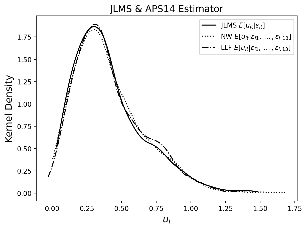
The first table reports the average estimated technical inefficiencies by the year as well as the average of their estimated standard deviations, which can be viewed as measures of the unexplained variation in \(u\). (We use a different random seed to Amsler et al. (2023) so our estimates are different from theirs.) Table 7.3 contains three predictors based on the panel model where the model parameters are estimated by MSLE. The JLMS estimator uses only the contemporaneous \(\epsilon_{it}\) in the conditioning set. The Nadaraya-Watson [NW] and Local Linear Forest [LLF] estimators use the expanded conditioning set and the APS14 approach to estimating the conditional expectation, described in Section 7.4.2. The second table contains three estimators based on the model with endogeneity where the parameters of the model are estimated by MSLE. For this part, we ignore the panel nature of the dataset (by viewing it as a pooled cross-section, i.e. by assuming independence over t as well as over i) and focus on the presence of the two types of inefficiency. In this case, JLMS is the estimator that does not use the $_{j}’s while NW and LLF include them in the conditioning set using the APS16 approach described in Section 7.6.1.
In the second table the average technical inefficiency score over all firms and years is similar across estimators, regardless of whether or not we condition on the allocative inefficiency terms. Over all years, the average standard deviation of technical inefficiency scores from the Local Linear Forest is considerably smaller than those from the JLMS or Nadaraya-Watson estimators. In Table 7.3, the mean technical inefficiency scores are always larger for all estimators and years in the data. Again, we find that the average technical inefficiency score over all firms and years is similar for all estimators. However, there are noticeable differences in the mean technical inefficiency score of estimators between years, for example in years 86, 87, 91 and 98. Finally, we note that the mean standard deviations for both non-parametric estimators are remarkably smaller than those associated with the JLMS estimator, suggesting that we explain a much larger portion of the unconditional variation in u. The technical inefficiency scores computed from the Local Linear Forest estimator are always associated with the smallest standard deviations.
Note: Users should uncomment the line calling the subprocess and change the file path to their own R executable location.
import numpy as np
import pandas as pd
import subprocess
import matplotlib.pyplot as plt

from scipy import stats
from scipy.linalg import expm, logm, norm
from scipy.optimize import minimize

def direct_mapping_mat(C):
    gamma = []

    try:
        # Check if input is of proper format: C is 2D np.array of suitable dimensions
        # and is positive-definite correlation matrix
        if not isinstance(C, np.ndarray):
            raise ValueError
        if C.ndim != 2:
            raise ValueError
        if C.shape[0] != C.shape[1]:
            raise ValueError
        if not all(
            [
                np.all(np.abs(np.diag(C) - np.ones(C.shape[0])) < 1e-8),
                np.all(np.linalg.eigvals(C) > 0),
                np.all(np.abs(C - C.T) < 1e-8),
            ]
        ):
            raise ValueError

        # Apply matrix log-transformation to C and get off-diagonal elements
        A = logm(C)
        gamma = A[np.triu_indices(C.shape[0], 1)]

    except ValueError:
        print("Error: input is of a wrong format")

    return gamma


def inverse_mapping_vec(gamma, tol_value=1e-8):
    C = []
    iter_number = -1

    # Check if input is of proper format: gamma is of suitable length
    if not isinstance(gamma, (np.ndarray, list)):
        raise ValueError
    if isinstance(gamma, np.ndarray):
        if gamma.ndim != 1:
            raise ValueError
    n = 0.5 * (1 + np.sqrt(1 + 8 * len(gamma)))
    if not all([n.is_integer(), n > 1]):
        raise ValueError

    # Check if tolerance value belongs to a proper interval
    # and change it to the default value otherwise
    if not (0 < tol_value <= 1e-4):
        tol_value = 1e-8
        print("Warning: tolerance value has been changed to default")

    # Place elements from gamma into off-diagonal parts
    # and put zeros on the main diagonal of [n x n] symmetric matrix A
    n = int(n)
    A = np.zeros(shape=(n, n))
    A[np.triu_indices(n, 1)] = gamma
    A = A + A.T

    # Read properties of the input matrix
    diag_vec = np.diag(A)  # get current diagonal
    diag_ind = np.diag_indices_from(
        A
    )  # get row and column indices of diagonal elements

    # Iterative algorithm to get the proper diagonal vector
    dist = np.sqrt(n)
    while dist > np.sqrt(n) * tol_value:
        diag_delta = np.log(np.diag(expm(A)))
        diag_vec = diag_vec - diag_delta
        A[diag_ind] = diag_vec
        dist = norm(diag_delta)
        iter_number += 1

    # Get a unique reciprocal correlation matrix
    C = expm(A)
    np.fill_diagonal(C, 1)

    return C

def Loglikelihood_Gaussian_copula_cross_sectional_application_SFA(theta, y, X, P, us_Sxn, n_inputs, S):

    n = len(y)

    alpha = np.exp(theta[0])
    beta = np.exp(theta[1:n_inputs+1])
    sigma2_v = theta[1+n_inputs]
    sigma2_u = theta[2+n_inputs]
    sigma2_w = np.exp(theta[3+n_inputs:(3+n_inputs)+(n_inputs-1)])
    mu_W = theta[(3+n_inputs)+(n_inputs-2)+1:(3+n_inputs)+(n_inputs-2)+(n_inputs)]

    rhos_log_form = theta[-3:]

    Rho_hat = inverse_mapping_vec(rhos_log_form)

    # Cobb-Douglas production function
    eps = y - np.log(alpha) - X@beta
    W = (np.tile(X[:, 0].reshape(-1, 1), (1, n_inputs-1)) - X[:,1:]) - (P[:,1:] - np.tile(P[:, 0].reshape(-1, 1), (1, n_inputs-1)) +(np.log(beta[0]) - np.log(beta[1:])))
    # Marginal density of allocative inefficiency terms
    Den_W = stats.norm.pdf(W, np.tile(mu_W, (n, 1)), np.tile(np.sqrt(sigma2_w), (n, 1)))
    CDF_W = stats.norm.cdf(W, np.tile(mu_W, (n, 1)), np.tile(np.sqrt(sigma2_w), (n, 1)))

    eps_Sxn = np.repeat(eps.reshape(-1,1), S, axis=1).T
    us_Sxn_scaled = np.sqrt(sigma2_u)*us_Sxn
    CdfUs = 2*(stats.norm.cdf(np.sqrt(sigma2_u)*us_Sxn, 0, np.sqrt(sigma2_u)) -0.5)
    eps_plus_us = eps_Sxn + us_Sxn_scaled
    den_eps_plus_us = stats.norm.pdf(eps_plus_us, 0, np.sqrt(sigma2_v))

    #Evaluate the integral via simulation (to integrate out u from eps+u)
    simulated_copula_pdfs = np.zeros((S,n))
    CDF_W_rep = {}
    for i in range(n_inputs-1):
        CDF_W_rep[i] = np.repeat(CDF_W[:, i].reshape(-1,1), S, axis=1).T

    for j in range(n):
        CDF_w_j = np.zeros((S, n_inputs-1))
        for i in range(n_inputs-1):
            CDF_w_j[:,i] = CDF_W_rep[i][:,j]
        U = np.concatenate([stats.norm.ppf(CdfUs[:, j]).reshape(-1,1),
                            stats.norm.ppf(CDF_w_j)],
                           axis=1)
        c123 = stats.multivariate_normal.pdf(U,
                                             mean = np.array([0, 0, 0]),
                                             cov=Rho_hat)/ np.prod(stats.norm.pdf(U), axis=1)
        simulated_copula_pdfs[:,j] = c123

    Integral = np.mean(simulated_copula_pdfs*den_eps_plus_us,
                       axis=0) #Evaluation of the integral over S simulated samples. Column-wise mean.
    # Joint desnity. product of marginal density of w_{i}, i = 1, ..., n_inputs and the joint density f(\epsilon, w)
    prod_Den_W = np.prod(Den_W, 1)
    DenAll = prod_Den_W*Integral;
    DenAll[DenAll < 1e-6] = 1e-6
    r = np.log(np.sum(beta))
    logDen = np.log(DenAll) + r
    logL = -np.sum(logDen)

    return logL

def estimate_Jondrow1982_u_hat(theta, n_inputs, n_corr_terms, y, X):

    alpha = theta[0]
    beta = theta[1:n_inputs+1]
    sigma2_v = theta[1+n_inputs]
    sigma2_u = theta[2+n_inputs]

    obs_eps = y - np.log(alpha) - X@beta
    _lambda = np.sqrt(sigma2_u/sigma2_v)
    sigma = np.sqrt(sigma2_u+sigma2_v)
    sig_star = np.sqrt(sigma2_u*sigma2_v/(sigma**2))
    u_hat = sig_star*(((stats.norm.pdf(_lambda*obs_eps/sigma))/(1-stats.norm.cdf(_lambda*obs_eps/sigma))) - ((_lambda*obs_eps)/sigma))
    V_u_hat = sig_star**2*(1+stats.norm.pdf(_lambda*obs_eps/sigma)/(1-stats.norm.cdf(_lambda*obs_eps/sigma))*_lambda*obs_eps/sigma-(stats.norm.pdf(_lambda*obs_eps/sigma)/(1-stats.norm.cdf(_lambda*obs_eps/sigma)))**2)

    return u_hat, V_u_hat

def Estimate_Jondrow1982_u_hat_panel_SFA_application_RS2007(alpha, beta, delta, sigma2_v, y, X, T, N):

    obs_eps = {}
    u_hat = np.zeros((N, T))
    V_u_hat = np.zeros((N, T))
    for t in range(T):
        sigma2_u = np.exp(delta[0] + delta[1]*t)
        _lambda = np.sqrt(sigma2_u)/np.sqrt(sigma2_v)
        sigma = np.sqrt(sigma2_u+sigma2_v)
        sig_star = np.sqrt(sigma2_u*sigma2_v/(sigma**2))

        u_hat_ = np.full(N, np.nan)
        V_u_hat_ = np.full(N, np.nan)
        obs_eps[t] = y[t] - np.log(alpha) - X[t]@beta # composed errors from the production function equation (i.e residuals from the production function)
        b = (obs_eps[t]*_lambda)/sigma
        u_hat_tmp = ((sigma*_lambda)/(1 + _lambda**2))*(stats.norm.pdf(b)/(1 - stats.norm.cdf(b)) - b)
        V_u_hat_tmp = sig_star**2*(1+stats.norm.pdf(b)/(1-stats.norm.cdf(b))*b-(stats.norm.pdf(b)/(1-stats.norm.cdf(b)))**2)

        u_hat_[:len(u_hat_tmp)] = u_hat_tmp
        V_u_hat_[:len(V_u_hat_tmp)] = V_u_hat_tmp
        u_hat[:, t] = u_hat_
        V_u_hat[:, t] = V_u_hat_

    return u_hat, V_u_hat

def simulate_error_components(Rho, n_inputs, S_kernel, seed):

    chol_of_rho = np.linalg.cholesky(Rho)
    Z = stats.multivariate_normal.rvs(mean=np.zeros(n_inputs),
                                      cov=np.eye(n_inputs),
                                      size=S_kernel,
                                      random_state=seed)
    X = chol_of_rho@Z.T
    U = stats.norm.cdf(X)

    return U.T

def Estimate_NW_u_hat_conditional_eps_panel_SFA_RS2007(theta, y, X, N, T, k, U_hat, S_kernel):

    alpha = theta[0]
    beta = theta[1:n_inputs+1]
    delta = theta[4:6]
    sigma2_v = theta[6]

    # Observed variables
    obs_eps = {}
    for t in range(T):
        eps__ = np.full(N, np.nan)
        tmp_eps = y[t] - np.log(alpha) - X[t]@beta
        eps__[:len(tmp_eps)] = tmp_eps
        obs_eps[t] = eps__

    # Simulated variables
    simulated_v = stats.multivariate_normal.rvs(mean=np.zeros(T),
                                                cov=np.eye(T)*sigma2_v,
                                                size=S_kernel) #simulate random noise for all T panels
    simulated_u = np.zeros((S_kernel, T))
    simulated_eps = np.zeros((S_kernel, T))
    for t in range(T):
        sigma2_u = np.exp(delta[0] + delta[1]*t)
        simulated_u[:, t] = np.sqrt(sigma2_u)*stats.norm.ppf((U_hat[:,t]+1)/2)
        simulated_eps[:,t] = simulated_v[:,t] - simulated_u[:,t]

    # Bandwidth information for each conditioning variable
    h_eps = np.zeros(T)
    for t in range(T):
        h_eps[t] = 1.06*S_kernel**(-1/5)*(max(np.std(simulated_eps[:,t]), stats.iqr(simulated_eps[:,t])/1.34))

    # kernel estimates for E[u_{t}|eps_{1}, ..., eps_{T}]
    # V[u|eps, w1, w2] = E[u^2|w2, w3, eps] - (E[u|w2, w3, eps])^2
    u_hat = np.zeros((N, T))
    u_hat2 = np.zeros((N, T))
    all_eps = np.concatenate([x.reshape(-1,1) for x in obs_eps.values()], axis=1)
    for i in range(N):
        obs_eps_i = all_eps[i, :]

        panel_i_kernel_regression_results = np.zeros(T)
        panel_i_kernel_regression_results2 = np.zeros(T)
        eps_kernel = np.zeros((S_kernel, T))
        # Construct the kernel distances for all T time periods
        for t in range(T):
            eps_kernel[:,t] = stats.norm.pdf((simulated_eps[:,t] - obs_eps[t][i])/h_eps[t])

        out = eps_kernel[:,np.all(~np.isnan(eps_kernel), axis=0)]
        kernel_product = np.prod(out, 1)
        for j in range(T): # NW for each t = 1, .., T observation in each panel i
            if not np.isnan(obs_eps_i[j]):
                panel_i_kernel_regression_results[j] = np.sum(kernel_product*simulated_u[:, j])/np.sum(kernel_product)
                panel_i_kernel_regression_results2[j] = np.sum(kernel_product*simulated_u[:,j]**2)/np.sum(kernel_product)
            else:
                panel_i_kernel_regression_results[j] = np.nan
                panel_i_kernel_regression_results2[j] = np.nan

        u_hat[i, :] = panel_i_kernel_regression_results
        u_hat2[i,  :] = panel_i_kernel_regression_results2

    V_u_hat = u_hat2 - (u_hat**2)

    return u_hat, V_u_hat

def Estimate_NW_u_hat_conditional_W_cross_sectional_application(theta, n_inputs, n_corr_terms, y, X, P, U_hat, S_kernel):

    n = len(y)

    alpha = theta[0]
    beta = theta[1:n_inputs+1]
    sigma2_v = theta[1+n_inputs]
    sigma2_u = theta[2+n_inputs]
    sigma2_w = np.exp(theta[3+n_inputs:(3+n_inputs)+(n_inputs-1)])
    mu_W = theta[(3+n_inputs)+(n_inputs-2)+1:(3+n_inputs)+(n_inputs-2)+(n_inputs)]

    # Observed variables
    obs_eps = y - np.log(alpha) - X@beta
    W = (np.tile(X[:, 0].reshape(-1, 1), (1, n_inputs-1)) - X[:,1:]) - (P[:,1:] - np.tile(P[:, 0].reshape(-1, 1), (1, n_inputs-1)) +(np.log(beta[0]) - np.log(beta[1:])))
    rep_obs_eps = np.repeat(obs_eps.reshape(-1,1), S_kernel, axis=1).T
    rep_obs_W = {}
    for i in range(n_inputs-1):
        rep_obs_W[i] = np.repeat(W[:, i].reshape(-1,1), S_kernel, axis=1).T

    # Simulated variables
    simulated_v = stats.norm.rvs(loc=0, scale=np.sqrt(sigma2_v), size=S_kernel)
    simulated_u = np.sqrt(sigma2_u)*stats.norm.ppf((U_hat[:, 0]+1)/2) # Simulated half normal rvs
    simulated_W = np.zeros((S_kernel, n_inputs-1))
    for i in range(n_inputs-1):
        simulated_W[:,i] = stats.norm.ppf(U_hat[:,i+1], mu_W[i], np.sqrt(sigma2_w[i]))
    simulated_eps = simulated_v - simulated_u

    # Bandwidth information for each conditioning variable
    h_eps = 1.06*S_kernel**(-1/5)*(max(np.std(simulated_eps), stats.iqr(simulated_eps)/1.34))
    h_W = np.zeros(n_inputs-1)
    for i in range(n_inputs-1):
        h_W[i] = 1.06*S_kernel**(-1/5)*(max(np.std(simulated_W[:,i]), stats.iqr(simulated_W[:,i])/1.34))
    h = np.concatenate([np.array([h_eps]), h_W])

    # Kernel estimates for E[u|eps, w1, w2]
    # V[u|eps, w1, w2] = E[u^2|w2, w3, eps] - (E[u|w2, w3, eps])^2
    kernel_regression_results1 = np.zeros(n)
    kernel_regression_results2 = np.zeros(n)
    for i in range(n):
        eps_kernel = stats.norm.pdf((simulated_eps - rep_obs_eps[:,i])/h[0])
        W_kernel = np.zeros((S_kernel,n_inputs-1))
        for j in range(n_inputs-1):
            W_kernel[:,j] = stats.norm.pdf((simulated_W[:,j] - rep_obs_W[j][:,i])/h[j+1])

        W_kernel_prod = np.prod(W_kernel, 1)
        kernel_product = eps_kernel*W_kernel_prod
        kernel_regression_results1[i] = np.sum(kernel_product*simulated_u)/np.sum(kernel_product)
        kernel_regression_results2[i] = np.sum(kernel_product*(simulated_u**2))/np.sum(kernel_product)

    u_hat = kernel_regression_results1
    V_u_hat = kernel_regression_results2 - (u_hat**2)

    return u_hat, V_u_hat

def Loglikelihood_APS14_dynamic_panel_SFA_u_RS2007(theta, y, X, N, T, k, S, FMSLE_us):

    if np.any(np.isnan(theta)):
        logDen = np.ones((n, 1))*-1e8
        logL = -np.sum(logDen)
    else:
        rhos = theta[7:]
        Rho = inverse_mapping_vec(rhos) # Gaussian copula correlation matrix

        alpha = np.exp(theta[0])
        beta = 1/(1+np.exp(-theta[1:4])) # Inverse logit transform of betas
        delta = theta[4:6]
        sigma2_v = theta[6]

        eps = {}
        for t in range(T):
            eps__ = np.full(N, np.nan)
            tmp_eps = y[t] - np.log(alpha) - X[t]@beta
            eps__[:len(tmp_eps)] = tmp_eps
            eps[t] = eps__

        if not np.all(np.linalg.eigvals(Rho) > 0):
            logDen = np.ones((n, 1))*-1e8
            logL = -np.sum(logDen)
        else:
            # Evaluate the integral via simulated MLE (FMSLE)
            A = np.linalg.cholesky(Rho)
            all_eps = np.concatenate([_eps.reshape(-1,1) for _eps in eps.values()], axis=1)
            FMSLE_densities = np.zeros(N)
            for i in range(N):
                eps_i = all_eps[i, :]
                n_NaNs = len(eps_i[np.isnan(eps_i)])
                eps_i = eps_i[~np.isnan(eps_i)] # remove any NaN from an unbalanced panel
                rep_eps_i = np.tile(eps_i, (S, 1))
                simulated_us_i = np.zeros((S, T))
                for t in range(T):
                   simulated_us_i[:, t] = FMSLE_us[t][:, i]

                # Transform simulated values to half-normal RV's
                CDF_u_i = stats.norm.cdf(simulated_us_i@A, np.zeros((S, T)), np.ones((S, T)))
                sigma2_u_hat = np.exp(delta[0] + delta[1]*np.arange(1, T+1, 1))
                u_i = stats.halfnorm.ppf(CDF_u_i,
                                         np.zeros((S, T)),
                                         np.tile(np.ones((1, T)) * np.sqrt(sigma2_u_hat), (S, 1)))

                # adjust for possible unbalanced panel
                u_i = u_i[:,:T-n_NaNs]
                # Joint density
                den_i = np.mean(stats.multivariate_normal.pdf(rep_eps_i + u_i,
                                                              mean=np.zeros(T-n_NaNs),
                                                          cov=np.eye(T-n_NaNs)*sigma2_v)) # eq 1 pg. 510 section 5.1 APS14
                if den_i < 1e-10:
                    den_i = 1e-10
                FMSLE_densities[i] = den_i

            logL = -np.sum(np.log(FMSLE_densities))

    return logL

def export_simulation_data_RS2007_electricity_application(theta, n_inputs, y, X, P, U_hat, S_kernel):

    alpha = theta[0]
    beta = theta[1:n_inputs+1]
    sigma2_v = theta[1+n_inputs]
    sigma2_u = theta[2+n_inputs]
    sigma2_w = np.exp(theta[3+n_inputs:(3+n_inputs)+(n_inputs-1)])
    mu_W = theta[(3+n_inputs)+(n_inputs-2)+1:(3+n_inputs)+(n_inputs-2)+(n_inputs)]

    # Observed variables
    obs_eps = y - np.log(alpha) - X@beta
    W = (np.tile(X[:, 0].reshape(-1, 1), (1, n_inputs-1)) - X[:,1:]) - (P[:,1:] - np.tile(P[:, 0].reshape(-1, 1), (1, n_inputs-1)) +(np.log(beta[0]) - np.log(beta[1:])))
    rep_obs_W = {}
    for i in range(n_inputs-1):
        rep_obs_W[i] = np.repeat(W[:, i].reshape(-1,1), S_kernel, axis=1).T

    # Simulated variables
    simulated_v = stats.norm.rvs(loc=0, scale=np.sqrt(sigma2_v), size=S_kernel)
    simulated_u = np.sqrt(sigma2_u)*stats.norm.ppf((U_hat[:, 0]+1)/2) # Simulated half normal rvs
    simulated_W = np.zeros((S_kernel, n_inputs-1))
    for i in range(n_inputs-1):
        simulated_W[:,i] = stats.norm.ppf(U_hat[:,i+1], mu_W[i], np.sqrt(sigma2_w[i]))
    simulated_eps = simulated_v - simulated_u

    # Export
    NN_train_eps_W = pd.DataFrame(np.concatenate([simulated_eps.reshape(-1,1), simulated_W],
                                                 axis=1),
                                  columns=['train_simulated_eps']+[f'train_simulated_w{i+1}' for i in range(n_inputs-1)])
    NN_train_u = pd.DataFrame(simulated_u,
                              columns=['train_simulated_u'])
    NN_test_eps_W = pd.DataFrame(np.concatenate([obs_eps.reshape(-1,1), W],
                                                 axis=1),
                                  columns=['test_simulated_eps']+[f'test_simulated_w{i+1}' for i in range(n_inputs-1)])

    NN_train_eps_W.to_csv(r'./cross_sectional_SFA_RS2007_electricity_application_NN_train_eps_W.csv',
                          index=False)
    NN_train_u.to_csv(r'./cross_sectional_SFA_RS2007_electricity_application_NN_train_u.csv',
                          index=False)
    NN_test_eps_W.to_csv(r'./cross_sectional_SFA_RS2007_electricity_application_NN_test_eps_W.csv',
                          index=False)

def export_RS2007_electricity_SFA_panel_data(theta, y, X, N, T, U_hat, S_kernel):

    alpha = theta[0]
    beta = theta[1:4]
    delta = theta[4:6]
    sigma2_v = theta[6]

    #Observed variables
    obs_eps = {}
    for t in range(T):
        eps__ = np.full(N, np.nan)
        tmp_eps = y[t] - np.log(alpha) - X[t]@beta
        eps__[:len(tmp_eps)] = tmp_eps
        obs_eps[t] = eps__

    obs_eps = np.concatenate([x.reshape(-1, 1) for x in obs_eps.values()], axis=1)

    # Simulated variables
    simulated_v = stats.multivariate_normal.rvs(np.zeros(T), np.eye(T)*sigma2_v, S_kernel) # simulate random noise for all T panels
    simulated_u = np.zeros((S_kernel, T))
    simulated_eps = np.zeros((S_kernel, T))
    for t in range(T):
        sigma2_u = np.exp(delta[0] + delta[1]*t)
        simulated_u[:, t] = np.sqrt(sigma2_u)*stats.norm.ppf((U_hat[:, t]+1)/2) # simulated half normal rvs
        simulated_eps[:, t] = simulated_v[:, t] - simulated_u[:, t]

    NN_train_eps = pd.DataFrame(simulated_eps,
                                columns=[f'train_eps_{t}' for t in range(T)])

    NN_train_u = pd.DataFrame(simulated_u,
                              columns=[f'train_u_{t}' for t in range(T)])

    NN_test_eps = pd.DataFrame(obs_eps,
                               columns=[f'test_eps_{t}' for t in range(T)])

    NN_train_eps.to_csv(r'./panel_SFA_RS2007_electricty_application_NN_train_eps.csv',
                          index=False)
    NN_train_u.to_csv(r'./panel_SFA_RS2007_electricty_application_NN_train_u.csv',
                          index=False)
    NN_test_eps.to_csv(r'./panel_SFA_RS2007_electricty_application_NN_test_eps.csv',
                          index=False)
data = pd.read_excel('steamelectric.xlsx')
data['fuel_price_index'] = np.nan
data.iloc[:-1, -1] = data.iloc[:-1, 2].values/data.iloc[1:,2].values
data['LM_price_index'] = np.nan
data.iloc[:-1, -1] = data.iloc[:-1, 3].values/data.iloc[1:,3].values
data.iloc[13:1007:14, :] = np.nan #drop last fuel price index for each plant
data = data.dropna()
X1 = (data['Fuel Costs ($1000)']/data['fuel_price_index'])*1000*1e-6; #fuel costs over price index
X2 = data['Operating Costs ($1000)']/data['LM_price_index']*1000*1e-6; #LM costs over price index
X3 = data['Capital ($1000)']/1000; # capital
X = np.log(pd.concat([X1, X2, X3], axis=1))
P = np.log(data[['fuel_price_index', 'LM_price_index', 'User Cost of Capital']])
y = np.log(data['Output (MWhr)']*1e-6) # output ml MWpH
# Estimate cross sectional models
n = len(y)
S = 500 # Number of Halton draws used in maximum simulated likelihood
S_kernel = 10000; # Number of simulated draws for evaluation of the conditional expectation
n_inputs = 3
n_corr_terms = ((n_inputs)^2-(n_inputs))/2 # Number of off diagonal lower triangular correlation/covariance terms for Gaussian copula correlation matrix.
initial_lalpha = -2.6
initial_beta = np.array([0.5, 0.3, 0.3])
initial_lbeta = np.log(initial_beta)
initial_logit_beta = np.log(initial_beta/(1-initial_beta))
initial_sigma2_v = 0.015
initial_lsigma2_v = np.log(initial_sigma2_v)
initial_sigma2_u = 0.15
initial_lsigma2_u = np.log(initial_sigma2_u)
initial_mu_W = np.array([0.5, 0])
sampler = stats.qmc.Halton(d=1,
scramble=True,
seed=123)
sample = sampler.random(n=n)
us_ = stats.norm.ppf((sample+1)/2, 0, 1)
us_Sxn = np.reshape(np.repeat(us_[:, np.newaxis], S, axis=1), (S, n))
# Gaussian Copula
initial_Sigma = np.array([[0.2, 0.09],
[0.09, 0.2]])
initial_sigma2_w = np.diag(initial_Sigma)
initial_lsigma2_w = np.log(initial_sigma2_w)
eps_ = y - initial_lalpha - X@initial_beta
W_ = (np.tile(X.iloc[:, 0].values.reshape(-1, 1), (1, n_inputs-1)) - X.iloc[:,1:].values) - (P.iloc[:,1:].values - np.tile(P.iloc[:, 0].values.reshape(-1, 1), (1, n_inputs-1)) +(np.log(initial_beta[0]) - np.log(initial_beta[1:])))
initial_Rho = np.corrcoef(np.concatenate([eps_.values.reshape(-1,1), W_], axis=1).T)
initial_lRho = direct_mapping_mat(initial_Rho)
Gaussian_copula_theta0 = np.concatenate([np.array([initial_lalpha]), initial_lbeta, np.array([initial_sigma2_v, initial_sigma2_u]),
initial_lsigma2_w, initial_mu_W, initial_lRho])
# Bounds to ensure sigma2v and sigma2u are >= 0
bounds = [(None, None) for x in range(4)] + [
(1e-5, np.inf),
(1e-5, np.inf),
] + [(None, None) for x in range(7)]
# Minimize the negative log-likelihood using numerical optimization.
MLE_results = minimize(
fun=Loglikelihood_Gaussian_copula_cross_sectional_application_SFA,
x0=Gaussian_copula_theta0,
method="L-BFGS-B",
tol = 1e-6,
options={"ftol": 1e-6, "maxiter": 1000, "maxfun": 6*1000},
args=(y.values, X.values, P.values, us_Sxn, n_inputs, S),
bounds=bounds,
)
Gaussian_copula_theta = MLE_results.x
logMLE = MLE_results.fun * -1 # Log-likelihood at the solution
# Transform parameters
Gaussian_copula_theta[:4] = np.exp(Gaussian_copula_theta[:4]) # Transform production system coefficients
Gaussian_copula_theta[6:8] = np.exp(Gaussian_copula_theta[6:8])
rhos_log_form = Gaussian_copula_theta[-3:]
Rho = inverse_mapping_vec(rhos_log_form)
Gaussian_copula_theta[-3:] = direct_mapping_mat(initial_Rho)
Rho_lower_trianglular = Rho[np.tril_indices(Rho.shape[1], 1)]
np.savetxt(r'./cross_sectional_SFA_RS2007_electricity_application_gaussian_copula_correlation_matrix.csv',
Rho,
delimiter=',')
# JLMS technical inefficiency scores
(Gaussian_copula_JLMS_u_hat,
Gaussian_copula_JLMS_V_u_hat) = estimate_Jondrow1982_u_hat(theta=Gaussian_copula_theta,
n_inputs=n_inputs,
n_corr_terms=n_corr_terms,
y=y.values,
X=X.values)
JLMS_u_hat_matrix = np.concatenate([data.loc[:, ['YEAR']].values, Gaussian_copula_JLMS_u_hat.reshape(-1,1)], axis=1)
JLMS_V_u_hat_matrix = np.concatenate([data.loc[:, ['YEAR']].values, Gaussian_copula_JLMS_V_u_hat.reshape(-1,1)], axis=1)
JLMS_u_hat_year_mean = np.zeros((13, 2))
JLMS_V_u_hat_year_mean = np.zeros((13, 2))
JLMS_std_u_hat_year_mean = np.zeros((13, 2))
for i, t in enumerate(range(86, 99)):
JLMS_u_hat_year_mean[i, 0] = t
JLMS_V_u_hat_year_mean[i, 0] = t
JLMS_std_u_hat_year_mean[i, 0] = t
JLMS_u_hat_year_mean[i, 1] = np.mean(JLMS_u_hat_matrix[JLMS_u_hat_matrix[:,0] == t, 1])
JLMS_V_u_hat_year_mean[i, 1] = np.mean(JLMS_V_u_hat_matrix[JLMS_V_u_hat_matrix[:,0] == t, 1])
JLMS_std_u_hat_year_mean[i, 1:] = np.mean(np.sqrt(JLMS_V_u_hat_matrix[JLMS_V_u_hat_matrix[:,0] == t, 1]))
# Copula Nadaraya Watson Scores
Gaussian_copula_U_hat = simulate_error_components(Rho=Rho,
n_inputs=n_inputs,
S_kernel=S_kernel,
seed=1234)
(Gaussian_copula_NW_conditional_W_u_hat,
Gaussian_copula_NW_conditional_W_V_u_hat) = Estimate_NW_u_hat_conditional_W_cross_sectional_application(theta=Gaussian_copula_theta,
n_inputs=n_inputs,
n_corr_terms=n_corr_terms,
y=y.values,
X=X.values,
P=P.values,
U_hat=Gaussian_copula_U_hat,
S_kernel=S_kernel)
NW_conditional_W_u_hat_matrix = np.concatenate([data.loc[:, ['YEAR']].values, Gaussian_copula_NW_conditional_W_u_hat.reshape(-1,1)], axis=1)
NW_conditional_W_V_u_hat_matrix = np.concatenate([data.loc[:, ['YEAR']].values, Gaussian_copula_NW_conditional_W_V_u_hat.reshape(-1,1)], axis=1)
NW_conditional_W_u_hat_year_mean = np.zeros((13, 2))
NW_conditional_W_V_u_hat_year_mean = np.zeros((13, 2))
NW_conditional_W_std_u_hat_year_mean = np.zeros((13, 2))
for i, t in enumerate(range(86, 99)):
NW_conditional_W_u_hat_year_mean[i, 0] = t
NW_conditional_W_V_u_hat_year_mean[i, 0] = t
NW_conditional_W_std_u_hat_year_mean[i, 0] = t
NW_conditional_W_u_hat_year_mean[i, 1] = np.mean(NW_conditional_W_u_hat_matrix[NW_conditional_W_u_hat_matrix[:,0] == t, 1])
NW_conditional_W_V_u_hat_year_mean[i, 1] = np.mean(NW_conditional_W_V_u_hat_matrix[NW_conditional_W_V_u_hat_matrix[:,0] == t, 1])
NW_conditional_W_std_u_hat_year_mean[i, 1] = np.mean(np.sqrt(NW_conditional_W_V_u_hat_matrix[NW_conditional_W_V_u_hat_matrix[:,0] == t, 1]))
# Export simulated training data and compute LLF u hat
export_simulation_data_RS2007_electricity_application(theta=Gaussian_copula_theta,
n_inputs=n_inputs,
y=y.values,
X=X.values,
P=P.values,
U_hat=Gaussian_copula_U_hat,
S_kernel=S_kernel)
# Users should change the first directory to the path where R is installed - use the code depending on your OS
# Windows
# subprocess.call([r'C:\Program Files\R\R-4.2.2\bin\Rscript.exe ./train_LocalLinear_forest_cross_sectional_RS2007_electricty_application.R'],
# shell=True)
# Mac
# subprocess.call([r'/usr/local/bin/Rscript', './train_LocalLinear_forest_cross_sectional_RS2007_electricty_application.R'])
Gaussian_copula_LLF_results = pd.read_csv(r'./LLF_Gaussian_copula_u_hat.csv')
Gaussian_copula_LLF_conditional_W_u_hat = Gaussian_copula_LLF_results.iloc[:,0].values
Gaussian_copula_LLF_conditional_W_V_u_hat = Gaussian_copula_LLF_results.iloc[:,1].values
LLF_u_hat_matrix = np.concatenate([data.loc[:, ['YEAR']].values, Gaussian_copula_LLF_conditional_W_u_hat.reshape(-1,1)], axis=1)
LLF_V_u_hat_matrix = np.concatenate([data.loc[:, ['YEAR']].values, Gaussian_copula_LLF_conditional_W_V_u_hat.reshape(-1,1)], axis=1)
LLF_u_hat_year_mean = np.zeros((13, 2))
LLF_V_u_hat_year_mean = np.zeros((13, 2))
LLF_std_u_hat_year_mean = np.zeros((13, 2))
for i, t in enumerate(range(86, 99)):
LLF_u_hat_year_mean[i, 0] = t
LLF_V_u_hat_year_mean[i, 0] = t
LLF_std_u_hat_year_mean[i, 0] = t
LLF_u_hat_year_mean[i, 1] = np.mean(LLF_u_hat_matrix[LLF_u_hat_matrix[:,0] == t, 1])
LLF_V_u_hat_year_mean[i, 1] = np.mean(LLF_V_u_hat_matrix[LLF_V_u_hat_matrix[:,0] == t, 1])
LLF_std_u_hat_year_mean[i, 1] = np.mean(np.sqrt(LLF_V_u_hat_matrix[LLF_V_u_hat_matrix[:,0] == t, 1]))
mean_Gaussian_copula_JLMS_u_hat = np.mean(Gaussian_copula_JLMS_u_hat)
mean_Gaussian_copula_JLMS_std_u_hat = np.mean(JLMS_std_u_hat_year_mean[:,1])
mean_Gaussian_copula_NW_conditional_W_u_hat = np.mean(Gaussian_copula_NW_conditional_W_u_hat)
mean_Gaussian_copula_NW_conditional_W_std_u_hat = np.mean(NW_conditional_W_std_u_hat_year_mean[:,1])
mean_Gaussian_copula_LLF_conditional_W_u_hat = np.mean(Gaussian_copula_LLF_conditional_W_u_hat);
mean_Gaussian_copula_LLF_conditional_W_std_u_hat = np.mean(LLF_std_u_hat_year_mean[:,1])
cross_sectional_results_table = pd.DataFrame(np.concatenate([np.array([x for x in range(86, 99)]).reshape(-1,1),
JLMS_u_hat_year_mean[:, [1]], JLMS_std_u_hat_year_mean[:, [1]],
NW_conditional_W_u_hat_year_mean[:, [1]], NW_conditional_W_std_u_hat_year_mean[:, [1]],
LLF_u_hat_year_mean[:, [1]], LLF_std_u_hat_year_mean[:, [1]]], axis=1),
columns=['Year', 'JLMS Est.', 'JLMS Std Dev', 'NW Est.', 'NW Std Dev', 'LLF Est.', 'LLF Std Dev'])
cross_sectional_averages = pd.DataFrame(np.array([mean_Gaussian_copula_JLMS_u_hat,
mean_Gaussian_copula_JLMS_std_u_hat,
mean_Gaussian_copula_NW_conditional_W_u_hat,
mean_Gaussian_copula_NW_conditional_W_std_u_hat,
mean_Gaussian_copula_LLF_conditional_W_u_hat,
mean_Gaussian_copula_LLF_conditional_W_std_u_hat]).reshape(1,-1),
columns=['JLMS Est.', 'JLMS Std Dev', 'NW Est.', 'NW Std Dev', 'LLF Est.', 'LLF Std Dev'],
index=['Average'])
print('Cross-Sectional Models (APS16 Estimator)')
display(cross_sectional_results_table)
display(cross_sectional_averages)Cross-Sectional Models (APS16 Estimator)| Year | JLMS Est. | JLMS Std Dev | NW Est. | NW Std Dev | LLF Est. | LLF Std Dev | |
|---|---|---|---|---|---|---|---|
| 0 | 86.0 | 0.460616 | 0.113611 | 0.453145 | 0.116160 | 0.459684 | 0.006971 |
| 1 | 87.0 | 0.395511 | 0.110433 | 0.400148 | 0.113094 | 0.399679 | 0.006790 |
| 2 | 88.0 | 0.389046 | 0.110389 | 0.388944 | 0.112926 | 0.395435 | 0.006410 |
| 3 | 89.0 | 0.342816 | 0.107974 | 0.345560 | 0.110662 | 0.348193 | 0.006073 |
| 4 | 90.0 | 0.376541 | 0.108117 | 0.375689 | 0.111443 | 0.382351 | 0.006412 |
| 5 | 91.0 | 0.382511 | 0.108342 | 0.382901 | 0.111295 | 0.389021 | 0.006524 |
| 6 | 92.0 | 0.404540 | 0.107777 | 0.403757 | 0.110551 | 0.408993 | 0.005997 |
| 7 | 93.0 | 0.413886 | 0.108060 | 0.408557 | 0.112749 | 0.417195 | 0.006726 |
| 8 | 94.0 | 0.391928 | 0.105610 | 0.389851 | 0.105226 | 0.400428 | 0.006062 |
| 9 | 95.0 | 0.406917 | 0.106064 | 0.411143 | 0.109713 | 0.415814 | 0.006120 |
| 10 | 96.0 | 0.379603 | 0.102596 | 0.377596 | 0.103694 | 0.387660 | 0.007358 |
| 11 | 97.0 | 0.348042 | 0.099227 | 0.351766 | 0.103336 | 0.356639 | 0.005932 |
| 12 | 98.0 | 0.357750 | 0.099781 | 0.358207 | 0.101077 | 0.364057 | 0.006379 |
| JLMS Est. | JLMS Std Dev | NW Est. | NW Std Dev | LLF Est. | LLF Std Dev | |
|---|---|---|---|---|---|---|
| Average | 0.388515 | 0.106768 | 0.388322 | 0.109379 | 0.394315 | 0.006443 |
# Estimate Panel data models
all_ = pd.concat([data[['Firm No', 'YEAR']], y, X], axis=1)
N = 72
T = len(all_['YEAR'].unique())
panel_y = {}
panel_X = {}
for j, t in enumerate(range(86, 99)):
    y__ = all_.loc[all_['YEAR'] == t, 'Output (MWhr)']
    X__ = all_.loc[all_['YEAR'] == t, [0, 1, 'Capital ($1000)']]
    panel_y[j] = y__.values
    panel_X[j] = X__.values

# Independent uniform random variables for FMSLE - assumes a Gaussian copula
sampler = stats.qmc.Halton(d=T,
                           scramble=True,
                           seed=123)
us_ = sampler.random(n=S)
us_ = stats.norm.ppf(us_) # transform to standard normal
FMSLE_us = {}
for t in range(T):
    us_Sxn = np.tile(us_[:, t-1][np.newaxis, :], (N, 1)).T
    FMSLE_us[t] = us_Sxn

initial_lalpha = -2.6
initial_beta = np.array([0.5, 0.2, 0.2])
initial_lbeta = np.log(initial_beta)
initial_logit_beta = np.log(initial_beta/(1-initial_beta))
initial_sigma2_v = 0.015
initial_lsigma2_v = np.log(initial_sigma2_v)
initial_sigma2_u = 0.15
initial_lsigma2_u = np.log(initial_sigma2_u)

initial_delta = np.array([initial_lsigma2_u, 0.2])
eps_ = {}
for t in range(T):
    eps__array = np.zeros(N)
    eps__ = panel_y[t] - initial_lalpha- panel_X[t]@initial_beta
    eps__array[:len(eps__)] = eps__
    eps_[t] = eps__array

k = len(initial_beta) + 1
initial_Rho = np.corrcoef(np.concatenate([eps.reshape(-1,1) for eps in eps_.values()], axis=1).T)
initial_lRho = direct_mapping_mat(initial_Rho)
theta0 = np.concatenate([np.array([initial_lalpha]),
                         initial_logit_beta,
                         initial_delta,
                         np.array([initial_sigma2_v]), initial_lRho])

# Bounds to ensure sigma2v and sigma2u are >= 0
bounds = [(None, None) for x in range(6)] + [
    (1e-5, np.inf),
] + [(None, None) for x in range(len(initial_lRho))]

# Minimize the negative log-likelihood using numerical optimization.
MLE_results = minimize(
    fun=Loglikelihood_APS14_dynamic_panel_SFA_u_RS2007,
    x0=theta0,
    method="L-BFGS-B",
    tol = 1e-8,
    options={"ftol": 1e-8, "maxiter": 1000, "maxfun": 35000, "maxcor": 500},
    args=(panel_y, panel_X, N, T, k, S, FMSLE_us),
    bounds=bounds,
)

APS14_theta = MLE_results.x
APS14_theta[0] = np.exp(APS14_theta[0])
APS14_theta[1:4] = 1/(1+np.exp(-APS14_theta[1:4])) # inverse logit transform of betas
APS14_logMLE = MLE_results.fun * -1

APS14_Rho = inverse_mapping_vec(APS14_theta[7:])
np.savetxt(r'./panel_SFA_RS2007_electricty_application_gaussian_copula_correlation_matrix.csv',
              APS14_Rho,
              delimiter=',')

# Simulated dependent U based upon estimated copula parameters
APS14_U_hat = simulate_error_components(Rho=APS14_Rho,
                                        n_inputs=T,
                                        S_kernel=S_kernel,
                                        seed=10)

# JLMS scores
(APS14_JLMS_u_hat,
 APS14_JLMS_V_u_hat) = Estimate_Jondrow1982_u_hat_panel_SFA_application_RS2007(alpha=APS14_theta[0],
                                                                               beta=APS14_theta[1:4],
                                                                               delta=APS14_theta[4:6],
                                                                               sigma2_v=APS14_theta[6],
                                                                               y=panel_y,
                                                                               X=panel_X,
                                                                               T=T,
                                                                               N=N)
APS14_JLMS_u_hat_year_mean = np.nanmean(APS14_JLMS_u_hat, axis=0)
APS14_JLMS_V_u_hat_year_mean = np.nanmean(APS14_JLMS_V_u_hat, axis=0)
APS14_JLMS_std_u_hat_year_mean = np.nanmean(np.sqrt(APS14_JLMS_V_u_hat), axis=0)

# Copula Nadaraya Watson
(APS14_NW_u_hat_conditional_eps,
 APS14_NW_V_u_hat_conditional_eps) = Estimate_NW_u_hat_conditional_eps_panel_SFA_RS2007(theta=APS14_theta,
                                                                                        y=panel_y,
                                                                                        X=panel_X,
                                                                                        N=N,
                                                                                        T=T,
                                                                                        k=k,
                                                                                        U_hat=APS14_U_hat,
                                                                                        S_kernel=S_kernel)
APS14_NW_u_hat_conditional_eps_year_mean = np.nanmean(APS14_NW_u_hat_conditional_eps, axis=0)
APS14_NW_V_u_hat_conditional_eps_year_mean = np.nanmean(APS14_NW_V_u_hat_conditional_eps, axis=0)
APS14_NW_std_u_hat_conditional_eps_year_mean = np.nanmean(np.sqrt(APS14_NW_V_u_hat_conditional_eps), axis=0)

export_RS2007_electricity_SFA_panel_data(theta=APS14_theta,
                                         y=panel_y,
                                         X=panel_X,
                                         N=N,
                                         T=T,
                                         U_hat=APS14_U_hat,
                                         S_kernel=S_kernel)

# Users should change the first directory to the path where R is installed
    # Windows
# subprocess.call(r'C:\Program Files\R\R-4.2.2\bin\Rscript.exe ./train_LocalLinear_forest_panel_RS2007_electricty_application.R',
#                 shell=True)
    # Mac
# subprocess.call([r'/usr/local/bin/Rscript', './train_LocalLinear_forest_panel_RS2007_electricty_application.R'])
APS14_LLF_conditional_eps_u_hat = pd.read_csv(r'./RS2007_electricity_LLF_Gaussian_copula_u_hat.csv')
APS14_LLF_conditional_eps_V_u_hat = pd.read_csv(r'./RS2007_electricity_LLF_Gaussian_copula_V_u_hat.csv')
APS14_LLF_conditional_eps_u_hat = APS14_LLF_conditional_eps_u_hat.iloc[:-1, :]
APS14_LLF_conditional_eps_V_u_hat = APS14_LLF_conditional_eps_V_u_hat.iloc[:-1, :]
APS14_LLF_conditional_eps_u_hat_year_mean = np.nanmean(APS14_LLF_conditional_eps_u_hat, axis=0)
APS14_LLF_conditional_eps_V_u_hat_year_mean = np.nanmean(APS14_LLF_conditional_eps_V_u_hat, axis=0)
APS14_LLF_conditional_eps_std_u_hat_year_mean = np.nanmean(np.sqrt(APS14_LLF_conditional_eps_V_u_hat), axis=0)

mean_Gaussian_copula_JLMS_u_hat = np.mean(APS14_JLMS_u_hat_year_mean)
mean_Gaussian_copula_JLMS_std_u_hat = np.mean(APS14_JLMS_std_u_hat_year_mean)
mean_Gaussian_copula_NW_conditional_W_u_hat = np.mean(APS14_NW_u_hat_conditional_eps_year_mean)
mean_Gaussian_copula_NW_conditional_W_std_u_hat = np.mean(APS14_NW_std_u_hat_conditional_eps_year_mean)
mean_Gaussian_copula_LLF_conditional_W_u_hat = np.mean(APS14_LLF_conditional_eps_u_hat_year_mean)
mean_Gaussian_copula_LLF_conditional_W_std_u_hat = np.mean(APS14_LLF_conditional_eps_std_u_hat_year_mean)

panel_results_table = pd.DataFrame(np.concatenate([np.array([x for x in range(86, 99)]).reshape(-1,1),
                                                APS14_JLMS_u_hat_year_mean.reshape(-1,1), APS14_JLMS_std_u_hat_year_mean.reshape(-1,1),
                                                APS14_NW_u_hat_conditional_eps_year_mean.reshape(-1,1), APS14_NW_std_u_hat_conditional_eps_year_mean.reshape(-1,1),
                                                APS14_LLF_conditional_eps_u_hat_year_mean.reshape(-1,1), APS14_LLF_conditional_eps_std_u_hat_year_mean.reshape(-1,1)], axis=1),
                                             columns=['Year', 'JLMS Est.', 'JLMS Std Dev', 'NW Est.', 'NW Std Dev', 'LLF Est.', 'LLF Std Dev'])
panel_averages = pd.DataFrame(np.array([mean_Gaussian_copula_JLMS_u_hat,
                                     mean_Gaussian_copula_JLMS_std_u_hat,
                                     mean_Gaussian_copula_NW_conditional_W_u_hat,
                                     mean_Gaussian_copula_NW_conditional_W_std_u_hat,
                                     mean_Gaussian_copula_LLF_conditional_W_u_hat,
                                     mean_Gaussian_copula_LLF_conditional_W_std_u_hat]).reshape(1,-1),
                                        columns=['JLMS Est.', 'JLMS Std Dev', 'NW Est.', 'NW Std Dev', 'LLF Est.', 'LLF Std Dev'],
                                        index=['Average'])
print('Panel Data Models (APS14 Estimator)')
display(panel_results_table)
display(panel_averages)
Panel Data Models (APS14 Estimator)| Year | JLMS Est. | JLMS Std Dev | NW Est. | NW Std Dev | LLF Est. | LLF Std Dev | |
|---|---|---|---|---|---|---|---|
| 0 | 86.0 | 0.511809 | 0.088466 | 0.408943 | 0.028140 | 0.424587 | 0.004156 |
| 1 | 87.0 | 0.404085 | 0.087483 | 0.418386 | 0.030822 | 0.432794 | 0.004808 |
| 2 | 88.0 | 0.438372 | 0.088059 | 0.433766 | 0.024779 | 0.429139 | 0.003546 |
| 3 | 89.0 | 0.416660 | 0.088250 | 0.440535 | 0.028039 | 0.434090 | 0.004797 |
| 4 | 90.0 | 0.404666 | 0.086727 | 0.457208 | 0.023650 | 0.460818 | 0.002694 |
| 5 | 91.0 | 0.409640 | 0.087197 | 0.465823 | 0.030365 | 0.470895 | 0.003679 |
| 6 | 92.0 | 0.407005 | 0.086893 | 0.387987 | 0.039109 | 0.388921 | 0.007091 |
| 7 | 93.0 | 0.412600 | 0.086621 | 0.415747 | 0.046351 | 0.432685 | 0.007462 |
| 8 | 94.0 | 0.385891 | 0.085183 | 0.404131 | 0.036672 | 0.410006 | 0.003713 |
| 9 | 95.0 | 0.414157 | 0.086411 | 0.396447 | 0.038572 | 0.401456 | 0.005797 |
| 10 | 96.0 | 0.374778 | 0.082006 | 0.366305 | 0.037658 | 0.368819 | 0.005441 |
| 11 | 97.0 | 0.332448 | 0.077521 | 0.323574 | 0.041057 | 0.331670 | 0.007950 |
| 12 | 98.0 | 0.381271 | 0.083361 | 0.382061 | 0.053896 | 0.386111 | 0.004549 |
| JLMS Est. | JLMS Std Dev | NW Est. | NW Std Dev | LLF Est. | LLF Std Dev | |
|---|---|---|---|---|---|---|
| Average | 0.407183 | 0.085706 | 0.407763 | 0.035316 | 0.41323 | 0.005053 |
# density plots
kde = stats.gaussian_kde(Gaussian_copula_JLMS_u_hat)
Gaussian_copula_JLMS_TE_kernel_x = np.linspace(Gaussian_copula_JLMS_u_hat.min(), Gaussian_copula_JLMS_u_hat.max(), 100)
Gaussian_copula_JLMS_TE_kernel = kde(Gaussian_copula_JLMS_TE_kernel_x)

kde = stats.gaussian_kde(Gaussian_copula_NW_conditional_W_u_hat)
Gaussian_copula_NW_TE_kernel_x = np.linspace(Gaussian_copula_JLMS_u_hat.min(), Gaussian_copula_JLMS_u_hat.max(), 100)
Gaussian_copula_NW_TE_kernel = kde(Gaussian_copula_NW_TE_kernel_x)

kde = stats.gaussian_kde(Gaussian_copula_LLF_conditional_W_u_hat)
Gaussian_copula_LLF_TE_kernel_x = np.linspace(Gaussian_copula_JLMS_u_hat.min(), Gaussian_copula_JLMS_u_hat.max(), 100)
Gaussian_copula_LLF_TE_kernel = kde(Gaussian_copula_LLF_TE_kernel_x)

figure = plt.Figure(figsize=(10,10))
plt.plot(Gaussian_copula_JLMS_TE_kernel_x, Gaussian_copula_JLMS_TE_kernel,
         color='k',
         ls='-',
         label=r'JLMS $E[u_{i}|\varepsilon_{i}]$')
plt.plot(Gaussian_copula_NW_TE_kernel_x,
         Gaussian_copula_NW_TE_kernel,
         ls=':',
         color='k',
         label=r'NW $E[u_{i}|\varepsilon_{i}, \omega_{i2}, \omega_{i3}]$')
plt.plot(Gaussian_copula_LLF_TE_kernel_x,
         Gaussian_copula_LLF_TE_kernel,
         ls='-.',
         color='k',
         label=r'LLF $E[u_{i}|\varepsilon_{i}, \omega_{i2}, \omega_{i3}]$')
plt.xlabel(r'$u_{i}$', fontsize=14)
plt.ylabel('Kernel Density', fontsize=14)
plt.title('JLMS & APS16 Estimator', fontsize=14)
plt.legend()
plt.show()

APS14_JLMS_u_hat_flat = APS14_JLMS_u_hat.flatten()
APS14_JLMS_u_hat_flat = APS14_JLMS_u_hat_flat[~np.isnan(APS14_JLMS_u_hat_flat)]
APS14_NW_u_hat_conditional_eps_flat = APS14_NW_u_hat_conditional_eps.flatten()
APS14_NW_u_hat_conditional_eps_flat = APS14_NW_u_hat_conditional_eps_flat[~np.isnan(APS14_NW_u_hat_conditional_eps_flat)]
APS14_LLF_conditional_eps_u_hat_flat = APS14_LLF_conditional_eps_u_hat.values.flatten()
APS14_LLF_conditional_eps_u_hat_flat = APS14_LLF_conditional_eps_u_hat_flat[~np.isnan(APS14_LLF_conditional_eps_u_hat_flat)]

kde = stats.gaussian_kde(APS14_JLMS_u_hat_flat)
APS14_JLMS_TE_kernel_x = np.linspace(APS14_JLMS_u_hat_flat.min(),
                                     APS14_JLMS_u_hat_flat.max(), 100)
APS14_JLMS_TE_kernel = kde(APS14_JLMS_TE_kernel_x)

kde = stats.gaussian_kde(APS14_NW_u_hat_conditional_eps_flat)
APS14_NW_TE_kernel_x = np.linspace(APS14_NW_u_hat_conditional_eps_flat.min(),
                                   APS14_NW_u_hat_conditional_eps_flat.max(), 100)
APS14_NW_TE_kernel = kde(APS14_NW_TE_kernel_x)

kde = stats.gaussian_kde(APS14_LLF_conditional_eps_u_hat_flat)
APS14_LLF_TE_kernel_x = np.linspace(APS14_LLF_conditional_eps_u_hat_flat.min(),
                                    APS14_LLF_conditional_eps_u_hat_flat.max(), 100)
APS14_LLF_TE_kernel = kde(APS14_LLF_TE_kernel_x)

figure = plt.Figure(figsize=(10,10))
plt.plot(APS14_JLMS_TE_kernel_x, APS14_JLMS_TE_kernel,
         color='k',
         ls='-',
         label=r'JLMS $E[u_{it}|\varepsilon_{it}]$')
plt.plot(APS14_NW_TE_kernel_x,
         APS14_NW_TE_kernel,
         ls=':',
         color='k',
         label=r'NW $E[u_{it}|\varepsilon_{i1}, \dots, \varepsilon_{i,13}]$')
plt.plot(APS14_LLF_TE_kernel_x,
         APS14_LLF_TE_kernel,
         ls='-.',
         color='k',
         label=r'LLF $E[u_{it}|\varepsilon_{i1}, \dots, \varepsilon_{i,13}]$')
plt.xlabel(r'$u_{i}$', fontsize=14)
plt.ylabel('Kernel Density', fontsize=14)
plt.title('JLMS & APS14 Estimator', fontsize=14)
plt.legend()
plt.show()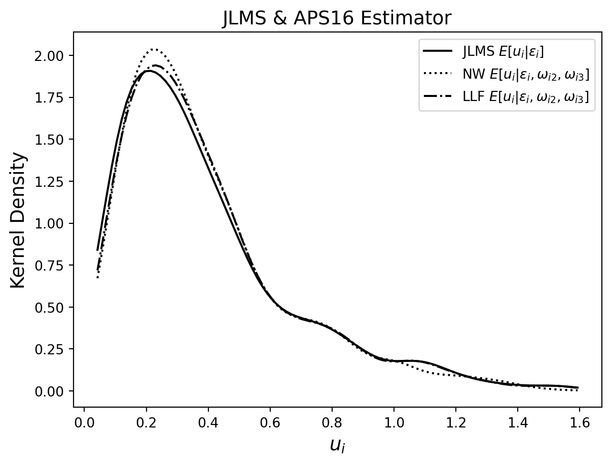
# Remove all previous function and variable definitions before the next exercise
%reset