import numpy as np
import seaborn as sns
from scipy import optimize, stats
from scipy.stats import spearmanr


def C12_conditional_u2(u1, u2, rho):
    return stats.multivariate_normal.cdf(
        (stats.norm.ppf(u1) - rho * stats.norm.ppf(u2)) / (np.sqrt(1 - rho**2))
    )


def root(z, u1, u2, rho):
return C12_conditional_u2(u1=z, u2=u2, rho=rho) - u14 Chapter 4: Copulas for panel stochastic frontier models
4.1 Exercise 4.1: Simulating from a Gaussian Copula
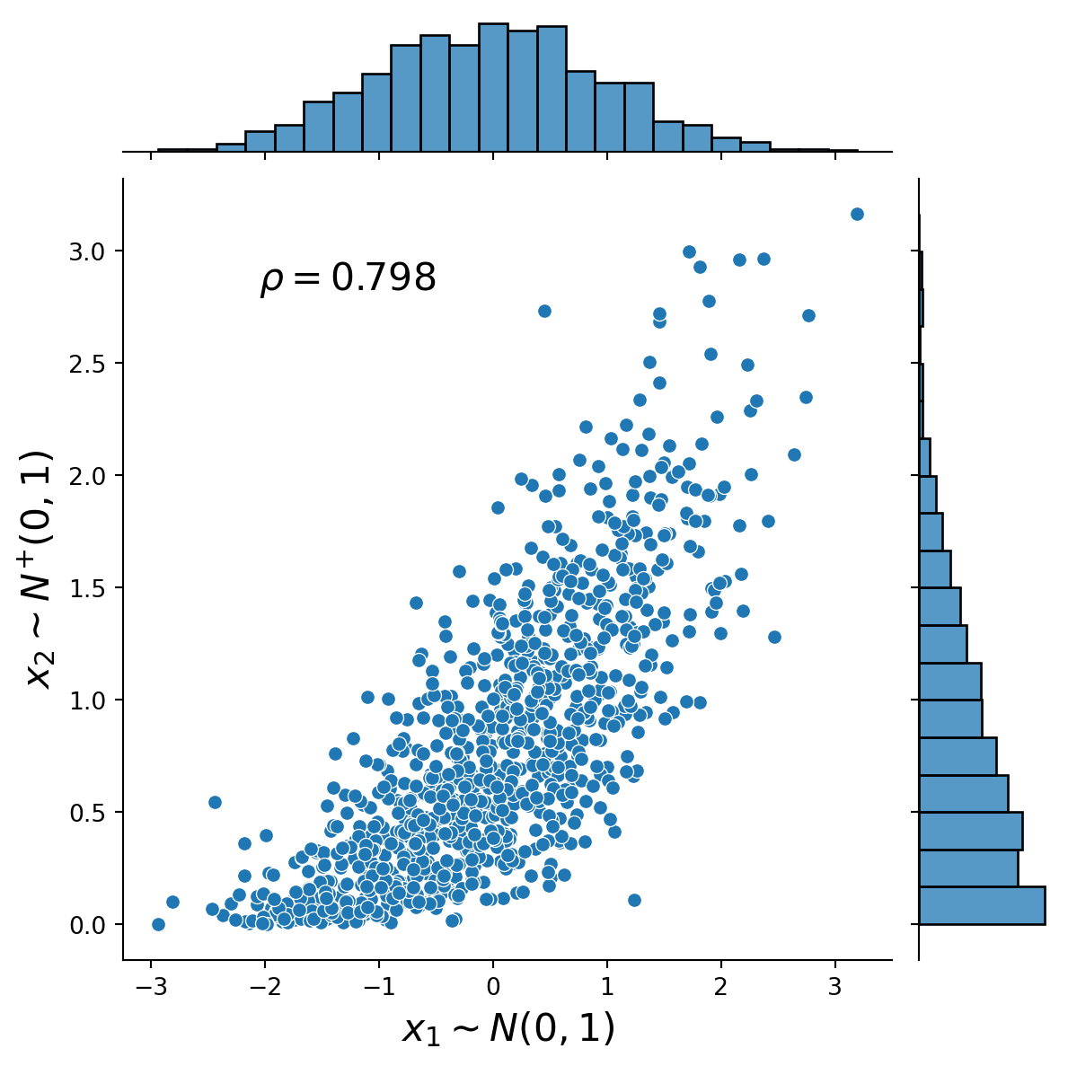
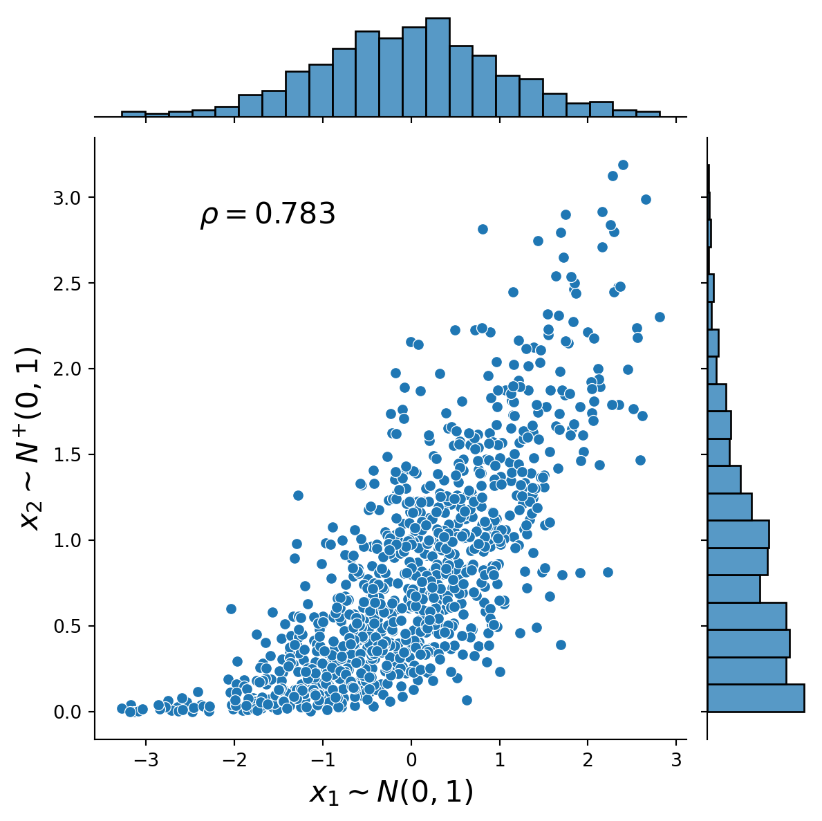
This exercise demonstrates how to simulate from a 2-dimensional Gaussian copula using the general Rosenblatt transform method (see, e.g. Joe, 2014, Chapter 6.9.1) and the Cholesky decomposition method (see, e.g., McNeil et al., 2015). The marginal distributions are normal and half-normal. The Figures present the distribution plots of the simulated dependent uniform random variables and the simulated dependent standard normal and half-normal random variables together with the associated value of Spearman’s rho.
rho = 0.8  # Dependence parameter of the Gaussian copula

# Rosenblatt transform approach
simulated_u1 = []
simulated_u2 = []
for i in range(1000):
    np.random.seed(i)
    uniforms = stats.uniform.rvs(size=2)
    u2 = uniforms[0]
    simulated_u2.append(u2)
    u1 = optimize.root_scalar(
        f=root, args=(uniforms[1], uniforms[0], rho), bracket=(0, 1)
    ).root
    simulated_u1.append(u1)

# Inverse transforms for the marginal distributions
x1 = stats.norm.ppf(simulated_u1)
x2 = stats.halfnorm.ppf(simulated_u2)

plot1 = sns.jointplot(x=simulated_u1, y=simulated_u2)
plot1.ax_joint.set_xlabel(r"$u_{1}$", fontsize=16)
plot1.ax_joint.set_ylabel(r"$u_{2}$", fontsize=16)
plot1.ax_joint.annotate(
    r"$\rho={}$".format(round(spearmanr(simulated_u1, simulated_u2)[0], 3)),
    xy=(0.2, 0.8),
    xycoords="figure fraction",
    fontsize=16,
)

plot2 = sns.jointplot(x=x1, y=x2)
plot2.ax_joint.set_xlabel(r"$x_{1} \sim N(0,1)$", fontsize=16)
plot2.ax_joint.set_ylabel(r"$x_{2} \sim N^{+}(0,1)$", fontsize=16)
plot2.ax_joint.annotate(
    r"$\rho={}$".format(round(spearmanr(x1, x2)[0], 3)),
    xy=(0.25, 0.75),
    xycoords="figure fraction",
    fontsize=16,
)
Text(0.25, 0.75, '$\\rho=0.798$')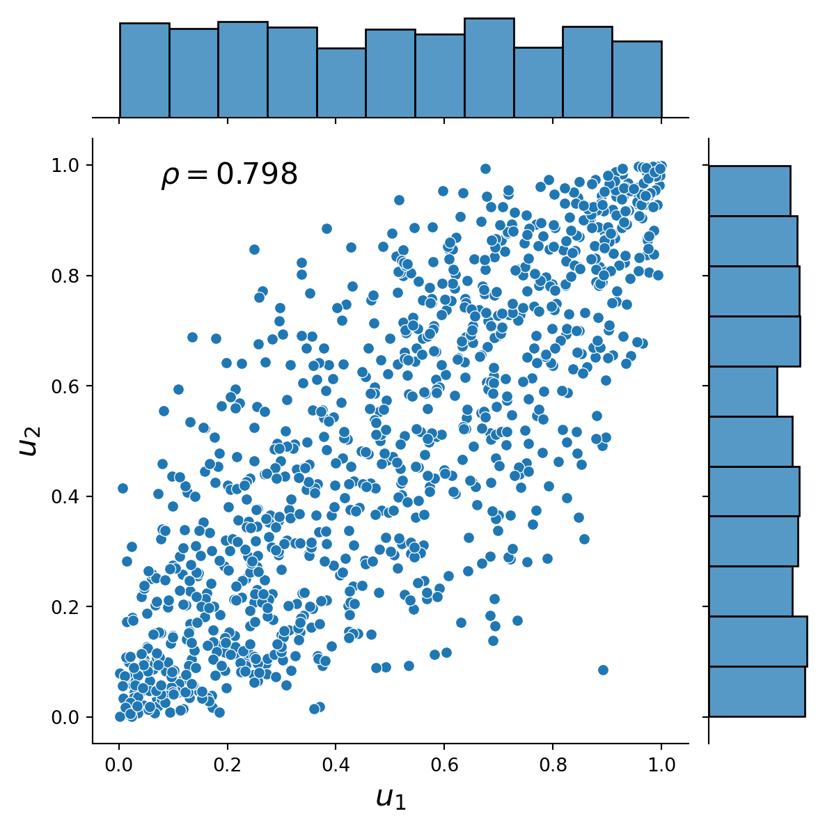
# Cholesky decomposition approach
P = np.array([[1, rho], [rho, 1]])
A = np.linalg.cholesky(P)
Z = stats.multivariate_normal.rvs(cov=np.eye(2), size=1000)
J = A @ Z.T
U = stats.norm.cdf(J).T

x1 = stats.norm.ppf(U[:, 0])
x2 = stats.halfnorm.ppf(U[:, 1])


plot1 = sns.jointplot(x=U[:, 0], y=U[:, 1])
plot1.ax_joint.set_xlabel(r"$u_{1}$", fontsize=16)
plot1.ax_joint.set_ylabel(r"$u_{2}$", fontsize=16)
plot1.ax_joint.annotate(
    r"$\rho={}$".format(round(spearmanr(U[:, 0], U[:, 1])[0], 3)),
    xy=(0.2, 0.8),
    xycoords="figure fraction",
    fontsize=16,
)

plot2 = sns.jointplot(x=x1, y=x2)
plot2.ax_joint.set_xlabel(r"$x_{1} \sim N(0,1)$", fontsize=16)
plot2.ax_joint.set_ylabel(r"$x_{2} \sim N^{+}(0,1)$", fontsize=16)
plot2.ax_joint.annotate(
    r"$\rho={}$".format(round(spearmanr(x1, x2)[0], 3)),
    xy=(0.25, 0.75),
    xycoords="figure fraction",
    fontsize=16,
)
Text(0.25, 0.75, '$\\rho=0.783$')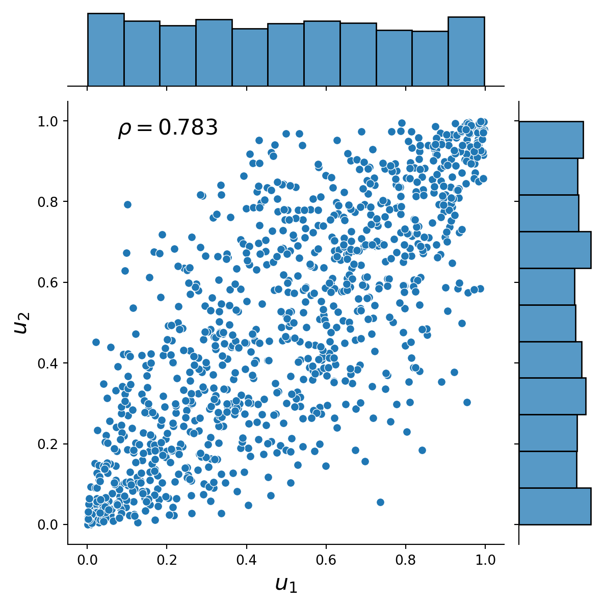
# Remove all previous function and variable definitions before the next exercise
%reset
4.2 Exercise 4.2: QMLE for Indonesian rice production
This exercise implements QMLE for a well-known data set of Indonesian rice farms see, e.g., Lee and Schmidt, 1993; Horrace and Schmidt, 1996, 2000). It contains data for 171 farmers with six annual observations of rice output (in kg), amount of seeds (kg), amount of urea (in kg), labor (in hours), land (in hectares), whether pesticides were used, which of thee rice varieties was planted and in which of six regions the farmer’s village is located.
Our results are based on all six cross sections. The robust standard errors we report for the QMLE account for potential correlation between the cross sections overtime. They are obtained using the “sandwich” formula, while the first set of standard errors are obtained using the estimated Hessian.
import numdifftools as nd
import numpy as np
import pandas as pd
from scipy import stats
from scipy.optimize import minimize


def log_density(coefs, y, X):
    # Get parameters
    alpha = coefs[0]
    beta = coefs[1:-2]
    sigma = coefs[-2]
    Lambda = coefs[-1]

    # Composed errors from the production function equation
    eps = y - alpha - X @ beta

    # Compute the log density
    # Note: stats.norm.pdf and stats.norm.cdf use loc=0 and scale=1 by default
    Den = (
        (2 / sigma)
        * stats.norm.pdf(eps / sigma)
        * stats.norm.cdf(-Lambda * eps / sigma)
    )
    logDen = np.log(Den)

    return logDen


def loglikelihood(coefs, y, X):
    # Obtain the log likelihood
    logDen = log_density(coefs, y, X)
    log_likelihood = -np.sum(logDen)

    return log_likelihood


def estimate(y, X):
    """
    Estimate model parameters by maximizing the log-likelihood function and compute standard errors.
    """
    # Starting values for MLE
    alpha = 5.5
    beta = [
        0.14,
        0.1,
        0.07,
        0.2,
        0.5,
        0.006,
        0.15,
        0.1,
        -0.06,
        -0.1,
        -0.1,
        -0.15,
        -0.05,
    ]
    sigma = 0.4
    _lambda = 1.3

    # Initial parameter vector
    theta0 = np.array([alpha] + beta + [sigma, _lambda])

    # Bounds to ensure sigma2v and sigma2u are >= 0
    bounds = [(None, None) for x in range(len(theta0) - 2)] + [
        (1e-5, np.inf),
        (1e-5, np.inf),
    ]

    # Minimize the negative log-likelihood using numerical optimization.
    MLE_results = minimize(
        fun=loglikelihood,
        x0=theta0,
        method="L-BFGS-B",
        options={"maxiter": 1000, "maxfun": 10000},
        args=(y, X),
        bounds=bounds,
    )

    theta = MLE_results.x  # Estimated parameter vector
    log_likelihood = MLE_results.fun * -1  # Log-likelihood at the solution

    # Estimate standard errors
    delta = 1e-6
    grad = np.zeros((len(y), len(theta)))
    for i in range(len(theta)):
        theta1 = np.copy(theta)
        theta1[i] += delta
        grad[:, i] = (log_density(theta1, y, X) - log_density(theta, y, X)) / delta

    OPG = grad.T @ grad  # Outer product of gradient
    ster = np.sqrt(np.diag(np.linalg.inv(OPG)))

    # Robust standard errors
    hessian = nd.Hessian(f=loglikelihood, method="central", step=1e-6)(theta, y, X)
    robust_ster = np.sqrt(
        np.diag(np.linalg.inv(-hessian) @ OPG @ np.linalg.inv(-hessian))
    )

    return theta, ster, robust_ster, log_likelihood
ricefarm = pd.read_csv(r"ricefarm.csv")
ricefarm = ricefarm.iloc[:, [0, 1, 3, 5, 6, 7, 8, 14, 16]]
# Create ID dummies
dar = np.round(ricefarm["ID"] / 100000).astype(int)
id_dummies = pd.get_dummies(dar, prefix="DR").astype(int)
ricefarm = pd.concat([ricefarm, id_dummies.iloc[:, :-1]], axis=1)
# Create rice variety dummies
rice_dummies = pd.get_dummies(ricefarm.iloc[:, 2], prefix="VAR").astype(int)
ricefarm = pd.concat([ricefarm, rice_dummies.iloc[:, 1:]], axis=1)
# Recode TSP as logs and zeros
ricefarm[ricefarm.columns[5]] = np.where(
ricefarm.iloc[:, 5] > 0, np.log(ricefarm.iloc[:, 5]), 0
)
# Convert pesticide usage to a dummy
ricefarm[ricefarm.columns[6]] = (ricefarm.iloc[:, 6] != 0).astype(int)
# Reorder the data
ricefarm = ricefarm.iloc[:, [8, 3, 4, 5, 7, 1, 6, 14, 15, 9, 10, 11, 12, 13]]
y = np.log(ricefarm.iloc[:, 0].values)
X = ricefarm.iloc[:, 1:].values
# Log covariates
X[:, 0:2] = np.log(X[:, 0:2])
X[:, 3] = np.log(X[:, 3])
X[:, 4] = np.log(X[:, 4])
theta, sterr, robust_ster, log_likelihood = estimate(y=y, X=X)
# Display the results as a table
results = pd.DataFrame(
data={"Est": theta, "St.Err": sterr, "Rob.St.Err.": robust_ster},
index=[
"CONST",
"SEED",
"UREA",
"TSP",
"LABOR",
"LAND",
"DP",
"DV1",
"DV2",
"DR1",
"DR2",
"DR3",
"DR4",
"DR5",
"SIGMA",
"LAMBDA",
],
)
results = results.round(4)
print("\nLL", round(log_likelihood, 3))
display(results)/Users/jleu0010/Documents/GitHub/EPA-Copula-SFA-website/venv/lib/python3.8/site-packages/pandas/core/arraylike.py:402: RuntimeWarning: divide by zero encountered in log
result = getattr(ufunc, method)(*inputs, **kwargs)
LL -342.322| Est | St.Err | Rob.St.Err. | |
|---|---|---|---|
| CONST | 5.5695 | 0.1746 | 0.2625 |
| SEED | 0.1451 | 0.0244 | 0.0327 |
| UREA | 0.1132 | 0.0142 | 0.0215 |
| TSP | 0.0763 | 0.0102 | 0.0122 |
| LABOR | 0.2004 | 0.0273 | 0.0312 |
| LAND | 0.4902 | 0.0237 | 0.0420 |
| DP | 0.0066 | 0.0285 | 0.0275 |
| DV1 | 0.1667 | 0.0387 | 0.0379 |
| DV2 | 0.1213 | 0.0588 | 0.0491 |
| DR1 | -0.0595 | 0.0532 | 0.0580 |
| DR2 | -0.1153 | 0.0532 | 0.0519 |
| DR3 | -0.1339 | 0.0378 | 0.0319 |
| DR4 | -0.1456 | 0.0350 | 0.0343 |
| DR5 | -0.0483 | 0.0420 | 0.0451 |
| SIGMA | 0.4430 | 0.0249 | 0.0309 |
| LAMBDA | 1.3592 | 0.2185 | 0.3871 |
# Save theta for use in exercise 5.3 and 5.5
np.savetxt("exercise_4_2_theta_python.txt", theta, delimiter=",")
# Remove all previous function and variable definitions before the next exercise
%reset4.3 Exercise 4.3: IQMLE of Indonesian rice production model
This exercise implements QMLE and two versions of IQMLE. The moment-based estimators have some theoretical advantages such as relatively higher asymptotic efficiency but, in practice, they may be infeasible. In this application, for example, we have 16 parameters, 6 time periods and only 171 cross sectional observations. The vector of moment conditions on which the IQMLE is based is 96×1. Obtaining stable GMM estimates for this problem with only 171 observations proved impossible.Therefore, instead of estimating the full vector of parameters we considered a simplified problem of estimating only two parameters, the constant and one slope coefficient, while keeping the other parameters constrained to be equal to their QMLE values. We therefore have 12 moment conditions to use in the IQMLE. This is a more appropriate setting for a moment-based estimation using a sample of size 171.
IQMLE-1 is the estimates obtained by the two-step GMM. In the first step, we obtain preliminary parameter estimates using the identity matrix for weighting. In the second step, we estimate the covariance matrix of the moment conditions and update the weighting by the inverse of the covariance matrix. IQMLE-2 is the iterated GMM estimation, in which we carry on the updating for 5 more iterations. The iterated GMM estimates are more efficient relative to the QMLE and the two-step GMM, which is evidenced by the slightly smaller standard errors of this estimate. On the other hand, the GMM estimators are known to have substantial small sample biases. The dispersion of the parameter estimates reported in the table suggests that these biases may be an issue here.
import numpy as np
import pandas as pd
from scipy import stats
from scipy.optimize import minimize
def criterion_function(theta, theta_fixed, W, y, X):
s = np.mean(mom(theta, theta_fixed, y, X), axis=0)
Qn = s.T @ W @ s
return Qn
def mom(theta, theta_fixed, y, X):
deriv = [] # Nx(Tx2) matrix of derivatives
for i in range(T):
# gradient of the density function w.r.t alpha and beta1 for cross section i
deriv.append(score(theta, theta_fixed, y[i], X[i]))
deriv_matrix = np.concatenate(deriv, axis=1)
return deriv_matrix
def score(theta, theta_fixed, y, X):
all_theta = np.concatenate([theta, theta_fixed])
beta = np.array(all_theta[:-2])
sigma = all_theta[-2]
_lambda = all_theta[-1]
xb = X @ beta
ind = (y - xb) / sigma
sc_beta_i = ind / sigma + stats.norm.pdf(ind * _lambda) * _lambda / sigma / (
1 - stats.norm.cdf(ind * _lambda)
)
sc_beta = np.diag(sc_beta_i) @ X[:, :2]
return sc_beta
def scorederiv(theta, theta_fixed, y, X):
deriv = []
for i in range(T):
# gradient of the density function w.r.t alpha and beta1 for cross section i
deriv.append(np.mean(score(theta, theta_fixed, y[i], X[i]), axis=0))
deriv_matrix = np.concatenate(deriv, axis=0)
return deriv_matrix
def estimate(y, X, theta_fixed):
"""
Estimate model parameters by maximizing the log-likelihood function and compute standard errors.
"""
N = 171
T = 6
# Starting values for MLE
alpha = 5.2
beta = 0.3
# Initial parameter vector
theta0 = [alpha, beta]
# Initial weighting matrix as the identity matrix
W_start = np.eye(len(theta0) * T)
# Minimize the negative log-likelihood using numerical optimization.
MLE_results = minimize(
fun=criterion_function,
x0=theta0,
method="Nelder-Mead",
options={"maxiter": 1000},
args=(theta_fixed, W_start, y, X),
)
for j in range(5):
revised_moments = mom(theta=MLE_results["x"], theta_fixed=theta_fixed, y=y, X=X)
C = (revised_moments.T @ revised_moments) / N
Wn = np.linalg.inv(C)
MLE_results = minimize(
fun=criterion_function,
x0=theta0,
method="Nelder-Mead",
options={"maxiter": 1000},
args=(theta_fixed, Wn, y, X),
)
if j == 0:
two_step_GMM_results = MLE_results
two_step_revised_moments = mom(
theta=MLE_results["x"], theta_fixed=theta_fixed, y=y, X=X
)
Wn_two_step_GMM = np.linalg.inv(
(two_step_revised_moments.T @ two_step_revised_moments) / N
)
iterated_GMM_results = MLE_results
Wn_iterated_GMM = Wn
two_step_GMM_theta = two_step_GMM_results["x"]
iterated_GMM_theta = iterated_GMM_results["x"]
# Estimate standard errors
delta = 1e-6
grad_two_step_GMM_results = np.zeros(
(len(theta0) * T, len(two_step_GMM_results["x"]))
)
grad_iterated_GMM_results = np.zeros(
(len(theta0) * T, len(iterated_GMM_results["x"]))
)
for i in range(len(theta0)):
theta1_iterated_GMM = np.copy(iterated_GMM_results["x"])
theta1_two_step_GMM = np.copy(two_step_GMM_results["x"])
theta1_iterated_GMM[i] += delta
theta1_two_step_GMM[i] += delta
grad_iterated_GMM_results[:, i] = (
scorederiv(theta=theta1_iterated_GMM, theta_fixed=theta_fixed, y=y, X=X)
- scorederiv(
theta=iterated_GMM_results["x"], theta_fixed=theta_fixed, y=y, X=X
)
) / delta
grad_two_step_GMM_results[:, i] = (
scorederiv(theta=theta1_two_step_GMM, theta_fixed=theta_fixed, y=y, X=X)
- scorederiv(
theta=two_step_GMM_results["x"], theta_fixed=theta_fixed, y=y, X=X
)
) / delta
OM_iterated_GMM = (
np.linalg.inv(
grad_iterated_GMM_results.T @ Wn_iterated_GMM @ grad_iterated_GMM_results
)
/ N
)
OM_two_step_GMM = (
np.linalg.inv(
grad_two_step_GMM_results.T @ Wn_two_step_GMM @ grad_two_step_GMM_results
)
/ N
)
ster_iterated_GMM = np.sqrt(np.diag(OM_iterated_GMM))
ster_two_step_GMM = np.sqrt(np.diag(OM_two_step_GMM))
return two_step_GMM_theta, iterated_GMM_theta, ster_two_step_GMM, ster_iterated_GMMricefarm = pd.read_csv(r"ricefarm.csv")
# Import theta vector from exercise 5.2
exercise_4_2_theta = np.loadtxt("exercise_4_2_theta_python.txt", delimiter=",")[
2:
] # keep everything except alpha and beta1
ricefarm = ricefarm.iloc[:, [0, 1, 3, 5, 6, 7, 8, 14, 16]]
# Create ID dummies
dar = np.round(ricefarm["ID"] / 100000).astype(int)
id_dummies = pd.get_dummies(dar, prefix="DR").astype(int)
ricefarm = pd.concat([ricefarm, id_dummies.iloc[:, :-1]], axis=1)
# Create rice variety dummies
rice_dummies = pd.get_dummies(ricefarm.iloc[:, 2], prefix="VAR").astype(int)
ricefarm = pd.concat([ricefarm, rice_dummies.iloc[:, 1:]], axis=1)
# Recode TSP as logs and zeros
ricefarm[ricefarm.columns[5]] = np.where(
ricefarm.iloc[:, 5] > 0, np.log(ricefarm.iloc[:, 5]), 0
)
# Convert pesticide usage to a dummy
ricefarm[ricefarm.columns[6]] = (ricefarm.iloc[:, 6] != 0).astype(int)
# Reorder the data
ricefarm = ricefarm.iloc[:, [8, 3, 4, 5, 7, 1, 6, 14, 15, 9, 10, 11, 12, 13]]
y = np.log(ricefarm.iloc[:, 0].values)
X = ricefarm.iloc[:, 1:].values
# Log covariates
X[:, 0:2] = np.log(X[:, 0:2])
X[:, 3] = np.log(X[:, 3])
X[:, 4] = np.log(X[:, 4])
X = np.concatenate([np.ones((len(X), 1)), X], axis=1)
# Cross sections of y and X
N = 171
T = 6
y_t = []
X_t = []
for t in range(T):
if t == 0:
y_t.append(y[:N])
X_t.append(X[:N, :])
else:
y_t.append(y[t * N : (t + 1) * N])
X_t.append(X[t * N : (t + 1) * N, :])
two_step_GMM_theta, iterated_GMM_theta, ster_two_step_GMM, ster_iterated_GMM = estimate(
y=y_t, X=X_t, theta_fixed=exercise_4_2_theta
)
# Display the results as a table
results = pd.DataFrame(
data={
"IQMLE-1 Est": two_step_GMM_theta,
"IQMLE-1 St.Err": ster_two_step_GMM,
"IQMLE-2 Est": iterated_GMM_theta,
"IQMLE-2 St.Err": ster_iterated_GMM,
},
index=["CONST", "SEED"],
)
results = results.round(4)
display(results)/Users/jleu0010/Documents/GitHub/EPA-Copula-SFA-website/venv/lib/python3.8/site-packages/pandas/core/arraylike.py:402: RuntimeWarning: divide by zero encountered in log
result = getattr(ufunc, method)(*inputs, **kwargs)| IQMLE-1 Est | IQMLE-1 St.Err | IQMLE-2 Est | IQMLE-2 St.Err | |
|---|---|---|---|---|
| CONST | 5.2154 | 0.0378 | 5.4842 | 0.0311 |
| SEED | 0.2871 | 0.0155 | 0.1716 | 0.0123 |
# Remove all previous function and variable definitions before the next exercise
%reset4.4 Exercise 4.4: Full MLE of the Indonesian rice production model
This exercise implements the FMLE estimator. We use the Gaussian copula to construct a multivariate distribution of εεε. The Gaussian copula is defined in Example45.1. In the Gaussian copula, the dependence structure between the marginals is represented by the correlation matrix \(R\). So our FMLE results contain estimates of a 6×6 correlation matrix, which are not reported. We use the correlation matrix parameterization of Archakov and Hansen (2021) in the numerical optimization routines.
NOTE: This code will take a long time to run because of the numerical integration routines required.
import multiprocessing
from itertools import product
import numpy as np
import pandas as pd
import scipy.integrate as integrate
from joblib import Parallel, delayed
from scipy import stats
from scipy.linalg import expm, logm, norm
from scipy.optimize import minimize
def direct_mapping_mat(C):
gamma = []
try:
# Check if input is of proper format: C is 2D np.array of suitable dimensions
# and is positive-definite correlation matrix
if not isinstance(C, np.ndarray):
raise ValueError
if C.ndim != 2:
raise ValueError
if C.shape[0] != C.shape[1]:
raise ValueError
if not all(
[
np.all(np.abs(np.diag(C) - np.ones(C.shape[0])) < 1e-8),
np.all(np.linalg.eigvals(C) > 0),
np.all(np.abs(C - C.T) < 1e-8),
]
):
raise ValueError
# Apply matrix log-transformation to C and get off-diagonal elements
A = logm(C)
gamma = A[np.triu_indices(C.shape[0], 1)]
except ValueError:
print("Error: input is of a wrong format")
return gamma
def ALS77_epsilon_density(eps, sigma, _lambda):
return (
(2 / sigma)
* stats.norm.pdf(eps / sigma)
* stats.norm.cdf(-_lambda * eps / sigma)
)
def inverse_mapping_vec(gamma, tol_value=1e-8):
C = []
iter_number = -1
# Check if input is of proper format: gamma is of suitable length
if not isinstance(gamma, (np.ndarray, list)):
raise ValueError
if isinstance(gamma, np.ndarray):
if gamma.ndim != 1:
raise ValueError
n = 0.5 * (1 + np.sqrt(1 + 8 * len(gamma)))
if not all([n.is_integer(), n > 1]):
raise ValueError
# Check if tolerance value belongs to a proper interval
# and change it to the default value otherwise
if not (0 < tol_value <= 1e-4):
tol_value = 1e-8
print("Warning: tolerance value has been changed to default")
# Place elements from gamma into off-diagonal parts
# and put zeros on the main diagonal of [n x n] symmetric matrix A
n = int(n)
A = np.zeros(shape=(n, n))
A[np.triu_indices(n, 1)] = gamma
A = A + A.T
# Read properties of the input matrix
diag_vec = np.diag(A) # get current diagonal
diag_ind = np.diag_indices_from(
A
) # get row and column indices of diagonal elements
# Iterative algorithm to get the proper diagonal vector
dist = np.sqrt(n)
while dist > np.sqrt(n) * tol_value:
diag_delta = np.log(np.diag(expm(A)))
diag_vec = diag_vec - diag_delta
A[diag_ind] = diag_vec
dist = norm(diag_delta)
iter_number += 1
# Get a unique reciprocal correlation matrix
C = expm(A)
np.fill_diagonal(C, 1)
return C
def integrate_ALS77(t, i, eps_it, sigma, _lambda):
return (
t,
i,
integrate.quad(
func=ALS77_epsilon_density, args=(sigma, _lambda), a=-4, b=eps_it
)[0],
)
def log_density(coefs, y, X):
N = 171
T = 6
n_corr_terms = int((T**2 - T) / 2)
# Get parameters
alpha = coefs[0]
beta = coefs[1:14]
gamma = coefs[14 : 14 + n_corr_terms]
sigma = coefs[-2]
_lambda = coefs[-1]
# Reconstruct the Gaussian copula correlation matrix
Rho = inverse_mapping_vec(gamma=gamma)
eps = np.zeros((N, T))
log_den_eps_margins = np.zeros((N, T)) # the log density of the margins
for t in range(T):
eps_t = y[t] - alpha - X[t] @ beta
eps[:, t] = eps_t
log_den_eps_margins[:, t] = np.log(
ALS77_epsilon_density(eps=eps_t, sigma=sigma, _lambda=_lambda)
)
# Compute F(eps_t) (CDF of epsion_t) by integrating the density over the interval (-4, eps)
eps_CDF = np.zeros((N, T))
jobs = product(range(T), range(N))
results = Parallel(n_jobs=multiprocessing.cpu_count())(
delayed(integrate_ALS77)(job[0], job[1], eps[job[1], job[0]], sigma, _lambda)
for job in jobs
)
for result in results:
eps_CDF[result[1], result[0]] = result[2]
eps_CDF[eps_CDF < 1e-4] = 1e-4
eps_CDF[eps_CDF > 0.999] = 0.999
# Compute the copula density for (eps_t, ..., eps_T)
log_copula_den = np.zeros(N)
for i in range(N):
log_copula_den[i] = np.log(
(1 / np.sqrt(np.linalg.det(Rho)))
* np.exp(
-0.5
* stats.norm.ppf(eps_CDF[i, :]).T
@ (np.linalg.inv(Rho) - np.eye(T))
@ stats.norm.ppf(eps_CDF[i, :])
)
)
# Compute the log density
logDen = log_copula_den + np.sum(log_den_eps_margins, axis=1)
return logDen
def loglikelihood(coefs, y, X):
# Obtain the log likelihood
logDen = log_density(coefs, y, X)
log_likelihood = -np.sum(logDen)
return log_likelihood
def estimate(y, X):
"""
Estimate model parameters by maximizing the log-likelihood function and compute standard errors.
"""
N = 171
T = 6
# Starting values for MLE
alpha = 5.5
beta = [0.1, 0.1, 0.06, 0.2, 0.5, 0.02, 0.1, 0.1, -0.1, -0.15, -0.1, -0.15, -0.05]
sigma = 0.45
_lambda = 1.2
# Initial values for the Gaussian copula correlation matrix
start_R = np.array(
[
[1.0000, 0.7837, 0.7724, 0.7202, 0.5778, 0.4978],
[0.7837, 1.0000, 0.6474, 0.8265, 0.4693, 0.5305],
[0.7724, 0.6474, 1.0000, 0.7030, 0.5933, 0.5297],
[0.7202, 0.8265, 0.7030, 1.0000, 0.5562, 0.5889],
[0.5778, 0.4693, 0.5933, 0.5562, 1.0000, 0.8475],
[0.4978, 0.5305, 0.5297, 0.5889, 0.8475, 1.0000],
]
)
gamma = direct_mapping_mat(C=start_R)
# Initial parameter vector
theta0 = np.array([alpha] + beta + gamma.tolist() + [sigma, _lambda])
# Bounds to ensure sigma2v and sigma2u are >= 0
bounds = [(None, None) for x in range(len(theta0) - 2)] + [
(1e-5, np.inf),
(1e-5, np.inf),
]
# Minimize the negative log-likelihood using numerical optimization.
MLE_results = minimize(
fun=loglikelihood,
x0=theta0,
method="L-BFGS-B",
options={"maxiter": 1000, "maxfun": 10000},
args=(y, X),
bounds=bounds,
)
theta = MLE_results.x # Estimated parameter vector
log_likelihood = MLE_results.fun * -1 # Log-likelihood at the solution
# Estimate standard errors
delta = 1e-6
grad = np.zeros((N, len(theta)))
for i in range(len(theta)):
theta1 = np.copy(theta)
theta1[i] += delta
grad[:, i] = (log_density(theta1, y, X) - log_density(theta, y, X)) / delta
OPG = grad.T @ grad # Outer product of gradient
ster = np.sqrt(np.diag(np.linalg.inv(OPG)))
# Only keep betas, sigma and lambda
theta = theta[:14].tolist() + theta[-2:].tolist()
ster = ster[:14].tolist() + ster[-2:].tolist()
return theta, ster, log_likelihoodricefarm = pd.read_csv(r"ricefarm.csv")
ricefarm = ricefarm.iloc[:, [0, 1, 3, 5, 6, 7, 8, 14, 16]]
# Create ID dummies
dar = np.round(ricefarm["ID"] / 100000).astype(int)
id_dummies = pd.get_dummies(dar, prefix="DR").astype(int)
ricefarm = pd.concat([ricefarm, id_dummies.iloc[:, :-1]], axis=1)
# Create rice variety dummies
rice_dummies = pd.get_dummies(ricefarm.iloc[:, 2], prefix="VAR").astype(int)
ricefarm = pd.concat([ricefarm, rice_dummies.iloc[:, 1:]], axis=1)
# Recode TSP as logs and zeros
ricefarm[ricefarm.columns[5]] = np.where(
ricefarm.iloc[:, 5] > 0, np.log(ricefarm.iloc[:, 5]), 0
)
# Convert pesticide usage to a dummy
ricefarm[ricefarm.columns[6]] = (ricefarm.iloc[:, 6] != 0).astype(int)
# Reorder the data
ricefarm = ricefarm.iloc[:, [8, 3, 4, 5, 7, 1, 6, 14, 15, 9, 10, 11, 12, 13]]
y = np.log(ricefarm.iloc[:, 0].values)
X = ricefarm.iloc[:, 1:].values
# Log covariates
X[:, 0:2] = np.log(X[:, 0:2])
X[:, 3] = np.log(X[:, 3])
X[:, 4] = np.log(X[:, 4])
# Cross sections of y and X
N = 171
T = 6
y_t = []
X_t = []
for t in range(T):
if t == 0:
y_t.append(y[:N])
X_t.append(X[:N, :])
else:
y_t.append(y[t * N : (t + 1) * N])
X_t.append(X[t * N : (t + 1) * N, :])
theta, ster, log_likelihood = estimate(y=y_t, X=X_t)
# Display the results as a table
results = pd.DataFrame(
data={"Est": theta, "St.Err": ster},
index=[
"CONST",
"SEED",
"UREA",
"TSP",
"LABOR",
"LAND",
"DP",
"DV1",
"DV2",
"DR1",
"DR2",
"DR3",
"DR4",
"DR5",
"SIGMA",
"LAMBDA",
],
)
results = results.round(4)
print("\nLL", round(log_likelihood, 3))
display(results)/Users/jleu0010/Documents/GitHub/EPA-Copula-SFA-website/venv/lib/python3.8/site-packages/pandas/core/arraylike.py:402: RuntimeWarning: divide by zero encountered in log
result = getattr(ufunc, method)(*inputs, **kwargs)
LL -261.689| Est | St.Err | |
|---|---|---|
| CONST | 5.4222 | 0.2134 |
| SEED | 0.1213 | 0.0230 |
| UREA | 0.1195 | 0.0166 |
| TSP | 0.0601 | 0.0143 |
| LABOR | 0.2184 | 0.0323 |
| LAND | 0.4909 | 0.0263 |
| DP | 0.0268 | 0.0285 |
| DV1 | 0.1379 | 0.0455 |
| DV2 | 0.1145 | 0.0608 |
| DR1 | -0.1085 | 0.0701 |
| DR2 | -0.1828 | 0.0690 |
| DR3 | -0.1195 | 0.0437 |
| DR4 | -0.1678 | 0.0449 |
| DR5 | -0.0872 | 0.0454 |
| SIGMA | 0.3959 | 0.0511 |
| LAMBDA | 0.7526 | 0.4648 |
# Remove all previous function and variable definitions before the next exercise
%reset4.5 Exercise 4.5: Copula-based GMM estimation of Indonesian rice production model
This exercise implements the copula-based GMM estimator We use the correlation matrix parameterization of Archakov and Hansen (2021) in the numerical optimization routines. As mentioned in Exercise 4.3, moment based estimators have some theoretical advantages such as relatively higher asymptotic efficiency but, in practice, they may be infeasible or unstable. For the GMM estimation in this application, we have 16 parameters, 6 time periods and only 171 cross sectional observations. The vector of moment conditions on which the GMM estimator is based contains the 96 moment conditions that come from the IQMLE plus the additional vector of copula-based moment conditions employed by the GMM estimator. That additional vector has 15 moment conditions for the parameters of R and 16 moment conditions for the parameters of the marginals. So we have as many as 127 moment conditions for the GMM estimator. Again, obtaining stable GMM estimates for this problem with only 171 observations proved impossible. As in Exercise 4.3, instead of estimating the full vector of parameters we considered the constrained problem of estimating only two parameters, the constant and one slope coefficient, with the other parameters fixed at their QMLE values. We therefore have 14 moment conditions to use in GMM, which is more appropriate for a moment based estimation using a sample of size 171.
import multiprocessing
from itertools import product
import numpy as np
import pandas as pd
import scipy.integrate as integrate
from joblib import Parallel, delayed
from scipy import stats
from scipy.linalg import expm, norm
from scipy.optimize import minimize
def inverse_mapping_vec(gamma, tol_value=1e-8):
C = []
iter_number = -1
# Check if input is of proper format: gamma is of suitable length
if not isinstance(gamma, (np.ndarray, list)):
raise ValueError
if isinstance(gamma, np.ndarray):
if gamma.ndim != 1:
raise ValueError
n = 0.5 * (1 + np.sqrt(1 + 8 * len(gamma)))
if not all([n.is_integer(), n > 1]):
raise ValueError
# Check if tolerance value belongs to a proper interval
# and change it to the default value otherwise
if not (0 < tol_value <= 1e-4):
tol_value = 1e-8
print("Warning: tolerance value has been changed to default")
# Place elements from gamma into off-diagonal parts
# and put zeros on the main diagonal of [n x n] symmetric matrix A
n = int(n)
A = np.zeros(shape=(n, n))
A[np.triu_indices(n, 1)] = gamma
A = A + A.T
# Read properties of the input matrix
diag_vec = np.diag(A) # get current diagonal
diag_ind = np.diag_indices_from(
A
) # get row and column indices of diagonal elements
# Iterative algorithm to get the proper diagonal vector
dist = np.sqrt(n)
while dist > np.sqrt(n) * tol_value:
diag_delta = np.log(np.diag(expm(A)))
diag_vec = diag_vec - diag_delta
A[diag_ind] = diag_vec
dist = norm(diag_delta)
iter_number += 1
# Get a unique reciprocal correlation matrix
C = expm(A)
np.fill_diagonal(C, 1)
return C
def ALS77_epsilon_density(eps, sigma, _lambda):
return (
(2 / sigma)
* stats.norm.pdf(eps / sigma)
* stats.norm.cdf(-_lambda * eps / sigma)
)
def integrate_ALS77(t, i, eps_it, sigma, _lambda):
return (
t,
i,
integrate.quad(
func=ALS77_epsilon_density, args=(sigma, _lambda), a=-4, b=eps_it
)[0],
)
def criterion_function(theta, theta_fixed, gamma_fixed, W, y, X):
s = np.mean(mom(theta, theta_fixed, gamma_fixed, y, X), axis=0)
Qn = s.T @ W @ s
return Qn
def mom(theta, theta_fixed, gamma_fixed, y, X):
N = 171
T = 6
# Marginals
marginal_deriv_matrix = [] # Nx(Tx2) matrix of
for i in range(T):
# gradient of the density function w.r.t alpha and beta1 for cross section i
marginal_deriv_matrix.append(score(theta, theta_fixed, y[i], X[i]))
marginal_deriv_matrix = np.concatenate(marginal_deriv_matrix, axis=1)
all_theta = np.concatenate([theta, theta_fixed])
beta = np.array(all_theta[:-2])
sigma = all_theta[-2]
_lambda = all_theta[-1]
eps = np.zeros((N, T))
eps_density = np.zeros((N, T)) # the log density of the margins
for t in range(T):
eps[:, t] = y[t] - X[t] @ beta
eps_density[:, t] = ALS77_epsilon_density(
eps=eps[:, t], sigma=sigma, _lambda=_lambda
)
# Compute F(eps_t) (CDF of epsion_t) by integrating the density over the interval (-4, eps)
eps_CDF = np.zeros((N, T))
jobs = product(range(T), range(N))
results = Parallel(n_jobs=multiprocessing.cpu_count())(
delayed(integrate_ALS77)(job[0], job[1], eps[job[1], job[0]], sigma, _lambda)
for job in jobs
)
for result in results:
eps_CDF[result[1], result[0]] = result[2]
eps_CDF[eps_CDF < 1e-4] = 1e-4
eps_CDF[eps_CDF > 0.999] = 0.999
scc1 = scorc(
eps_CDF=eps_CDF, eps_density=eps_density, i=0, gamma_fixed=gamma_fixed, X=X
)
scc2 = scorc(
eps_CDF=eps_CDF, eps_density=eps_density, i=1, gamma_fixed=gamma_fixed, X=X
)
deriv_matrix = np.concatenate([marginal_deriv_matrix, scc1, scc2], axis=1)
return deriv_matrix
def scorc(eps_CDF, eps_density, i, gamma_fixed, X):
T = 6
R = inverse_mapping_vec(gamma_fixed)
X_var = np.concatenate([X[t][:, i].reshape(-1, 1) for t in range(T)], axis=1)
if i == 0:
sc = np.sum(
1
/ stats.norm.pdf(eps_CDF).T
* eps_density.T
* ((np.linalg.inv(R) - np.eye(T)) @ eps_CDF.T),
0,
)
else:
sc = np.sum(
1
/ stats.norm.pdf(eps_CDF).T
* eps_density.T
* X_var.T
* ((np.linalg.inv(R) - np.eye(T)) @ eps_CDF.T),
0,
)
return sc.reshape(-1, 1)
def score(theta, theta_fixed, y, X):
all_theta = np.concatenate([theta, theta_fixed])
beta = np.array(all_theta[:-2])
sigma = all_theta[-2]
_lambda = all_theta[-1]
xb = X @ beta
ind = (y - xb) / sigma
sc_beta_i = ind / sigma + stats.norm.pdf(ind * _lambda) * _lambda / sigma / (
1 - stats.norm.cdf(ind * _lambda)
)
sc_beta = np.diag(sc_beta_i) @ X[:, :2]
return sc_beta
def scorederiv(theta, theta_fixed, gamma_fixed, y, X):
marginal_deriv_matrix = [] # Nx(Tx2) matrix of
for i in range(T):
# gradient of the density function w.r.t alpha and beta1 for cross section i
marginal_deriv_matrix.append(
np.mean(score(theta, theta_fixed, y[i], X[i]), axis=0)
)
marginal_deriv_matrix = np.concatenate(marginal_deriv_matrix, axis=0)
all_theta = np.concatenate([theta, theta_fixed])
beta = np.array(all_theta[:-2])
sigma = all_theta[-2]
_lambda = all_theta[-1]
eps = np.zeros((N, T))
eps_density = np.zeros((N, T)) # the log density of the margins
for t in range(T):
eps[:, t] = y[t] - X[t] @ beta
eps_density[:, t] = ALS77_epsilon_density(
eps=eps[:, t], sigma=sigma, _lambda=_lambda
)
# Compute F(eps_t) (CDF of epsion_t) by integrating the density over the interval (-4, eps)
eps_CDF = np.zeros((N, T))
jobs = product(range(T), range(N))
results = Parallel(n_jobs=multiprocessing.cpu_count())(
delayed(integrate_ALS77)(job[0], job[1], eps[job[1], job[0]], sigma, _lambda)
for job in jobs
)
for result in results:
eps_CDF[result[1], result[0]] = result[2]
eps_CDF[eps_CDF < 1e-4] = 1e-4
eps_CDF[eps_CDF > 0.999] = 0.999
scc1 = np.mean(
scorc(
eps_CDF=eps_CDF, eps_density=eps_density, i=0, gamma_fixed=gamma_fixed, X=X
),
axis=0,
)
scc2 = np.mean(
scorc(
eps_CDF=eps_CDF, eps_density=eps_density, i=1, gamma_fixed=gamma_fixed, X=X
),
axis=0,
)
deriv_matrix = np.concatenate([marginal_deriv_matrix, scc1, scc2], axis=0)
return deriv_matrix
def estimate(y, X, theta_fixed, gamma_fixed):
"""
Estimate model parameters by maximizing the log-likelihood function and compute standard errors.
"""
N = 171
T = 6
# Starting values for MLE
alpha = 5.2
beta = 0.3
# Initial parameter vector
theta0 = [alpha, beta]
# Initial weighting matrix as the identity matrix
W_start = np.eye(len(theta0) * T + 2)
# Minimize the negative log-likelihood using numerical optimization.
MLE_results = minimize(
fun=criterion_function,
x0=theta0,
method="Nelder-Mead",
options={"maxiter": 1000},
args=(theta_fixed, gamma_fixed, W_start, y, X),
)
for j in range(7):
revised_moments = mom(
theta=MLE_results["x"],
theta_fixed=theta_fixed,
gamma_fixed=gamma_fixed,
y=y,
X=X,
)
C = (revised_moments.T @ revised_moments) / N
Wn = np.linalg.inv(C)
MLE_results = minimize(
fun=criterion_function,
x0=theta0,
method="L-BFGS-B",
options={"maxiter": 1000},
args=(theta_fixed, gamma_fixed, Wn, y, X),
)
if j == 3:
two_step_GMM_results = MLE_results
two_step_revised_moments = mom(
theta=MLE_results["x"],
theta_fixed=theta_fixed,
gamma_fixed=gamma_fixed,
y=y,
X=X,
)
Wn_two_step_GMM = np.linalg.inv(
(two_step_revised_moments.T @ two_step_revised_moments) / N
)
iterated_GMM_results = MLE_results
Wn_iterated_GMM = Wn
two_step_GMM_theta = two_step_GMM_results["x"]
iterated_GMM_theta = iterated_GMM_results["x"]
# Estimate standard errors
delta = 1e-6
grad_two_step_GMM_results = np.zeros(
(len(theta0) * T + 2, len(two_step_GMM_results["x"]))
)
grad_iterated_GMM_results = np.zeros(
(len(theta0) * T + 2, len(iterated_GMM_results["x"]))
)
for i in range(len(theta0)):
theta1_iterated_GMM = np.copy(iterated_GMM_results["x"])
theta1_two_step_GMM = np.copy(two_step_GMM_results["x"])
theta1_iterated_GMM[i] += delta
theta1_two_step_GMM[i] += delta
grad_iterated_GMM_results[:, i] = (
scorederiv(
theta=theta1_iterated_GMM,
theta_fixed=theta_fixed,
gamma_fixed=gamma_fixed,
y=y,
X=X,
)
- scorederiv(
theta=iterated_GMM_results["x"],
theta_fixed=theta_fixed,
gamma_fixed=gamma_fixed,
y=y,
X=X,
)
) / delta
grad_two_step_GMM_results[:, i] = (
scorederiv(
theta=theta1_two_step_GMM,
theta_fixed=theta_fixed,
gamma_fixed=gamma_fixed,
y=y,
X=X,
)
- scorederiv(
theta=two_step_GMM_results["x"],
theta_fixed=theta_fixed,
gamma_fixed=gamma_fixed,
y=y,
X=X,
)
) / delta
OM_iterated_GMM = (
np.linalg.inv(
grad_iterated_GMM_results.T @ Wn_iterated_GMM @ grad_iterated_GMM_results
)
/ N
)
OM_two_step_GMM = (
np.linalg.inv(
grad_two_step_GMM_results.T @ Wn_two_step_GMM @ grad_two_step_GMM_results
)
/ N
)
ster_iterated_GMM = np.sqrt(np.diag(OM_iterated_GMM))
ster_two_step_GMM = np.sqrt(np.diag(OM_two_step_GMM))
return two_step_GMM_theta, iterated_GMM_theta, ster_two_step_GMM, ster_iterated_GMMricefarm = pd.read_csv(r"ricefarm.csv")
exercise_4_3_theta = np.loadtxt("exercise_4_2_theta_python.txt", delimiter=",")[
2:
] # keep everything except alpha and beta1
exercise_4_4_gamma = np.loadtxt("exercise_4_4_gamma_python.txt", delimiter=",")
ricefarm = ricefarm.iloc[:, [0, 1, 3, 5, 6, 7, 8, 14, 16]]
# Create ID dummies
dar = np.round(ricefarm["ID"] / 100000).astype(int)
id_dummies = pd.get_dummies(dar, prefix="DR").astype(int)
ricefarm = pd.concat([ricefarm, id_dummies.iloc[:, :-1]], axis=1)
# Create rice variety dummies
rice_dummies = pd.get_dummies(ricefarm.iloc[:, 2], prefix="VAR").astype(int)
ricefarm = pd.concat([ricefarm, rice_dummies.iloc[:, 1:]], axis=1)
# Recode TSP as logs and zeros
ricefarm[ricefarm.columns[5]] = np.where(
ricefarm.iloc[:, 5] > 0, np.log(ricefarm.iloc[:, 5]), 0
)
# Convert pesticide usage to a dummy
ricefarm[ricefarm.columns[6]] = (ricefarm.iloc[:, 6] != 0).astype(int)
# Reorder the data
ricefarm = ricefarm.iloc[:, [8, 3, 4, 5, 7, 1, 6, 14, 15, 9, 10, 11, 12, 13]]
y = np.log(ricefarm.iloc[:, 0].values)
X = ricefarm.iloc[:, 1:].values
# Log covariates
X[:, 0:2] = np.log(X[:, 0:2])
X[:, 3] = np.log(X[:, 3])
X[:, 4] = np.log(X[:, 4])
X = np.concatenate([np.ones((len(X), 1)), X], axis=1)
# Cross sections of y and X
N = 171
T = 6
y_t = []
X_t = []
for t in range(T):
if t == 0:
y_t.append(y[:N])
X_t.append(X[:N, :])
else:
y_t.append(y[t * N : (t + 1) * N])
X_t.append(X[t * N : (t + 1) * N, :])
two_step_GMM_theta, iterated_GMM_theta, ster_two_step_GMM, ster_iterated_GMM = estimate(
y=y_t, X=X_t, theta_fixed=exercise_4_3_theta, gamma_fixed=exercise_4_4_gamma
)
# Display the results as a table
results = pd.DataFrame(
data={
"IQMLE-1 Est": two_step_GMM_theta,
"IQMLE-1 St.Err": ster_two_step_GMM,
"IQMLE-2 Est": iterated_GMM_theta,
"IQMLE-2 St.Err": ster_iterated_GMM,
},
index=["CONST", "SEED"],
)
results = results.round(4)
display(results)/Users/jleu0010/Documents/GitHub/EPA-Copula-SFA-website/venv/lib/python3.8/site-packages/pandas/core/arraylike.py:402: RuntimeWarning: divide by zero encountered in log
result = getattr(ufunc, method)(*inputs, **kwargs)| IQMLE-1 Est | IQMLE-1 St.Err | IQMLE-2 Est | IQMLE-2 St.Err | |
|---|---|---|---|---|
| CONST | 5.0724 | 0.0432 | 5.2976 | 0.0372 |
| SEED | 0.3673 | 0.0183 | 0.2843 | 0.0157 |
# Remove all previous function and variable definitions before the next exercise
%reset4.6 Exercise 4.6: Quantiles at desired level of precision
import numpy as np
import pandas as pd
from scipy import stats
from scipy import integrate

def density_function(x, _lambda):

    density = 2/1*stats.norm.pdf(x/1)*stats.norm.cdf(-x*_lambda/1)

    return density

lambda_range = np.arange(0, 1.1, 0.1)
lb = -4
ub = 4
fine = 100000

quantiles = [0.1, 0.2, 0.3, 0.4, 0.5, 0.6, 0.7, 0.8, 0.9]
table = np.zeros((len(lambda_range), len(quantiles)))

y = np.arange(-4, 4+(ub-lb)/fine, (ub-lb)/fine)
for i in range(len(lambda_range)):
    F = np.zeros(len(y))
    for j in range(len(y)):
        F[j] = integrate.quad(density_function, lb, y[j], args=(lambda_range[i]))[0]
    lambda_qs = np.zeros(len(quantiles))
    for q in range(len(quantiles)):
        idx = np.argmin(np.abs(F-quantiles[q]))
        lambda_qs[q] = y[idx]
    table[i, :] = lambda_qs

# FINISH TABLE PLOTTING HERE
# Remove all previous function and variable definitions before the next exercise
%reset4.7 Exercise 4.7: Full MSLE of Indonesian rice farm production model
This Exercise implements FMSLE, where we use the Gaussian copula to construct and sample from a multivariate distribution of \(u\). We use \(S=1000\) draws in evaluating \(\hat{f}_{{\epsilon}}({\epsilon})\) by simulation. As in FMLE, the results include 15 estimated correlations. Now, these are correlations over \(t\) of \(\Phi^{-1}(F_u(u_t))\), not of \(\Phi^{-1}(F_\varepsilon(\varepsilon_t))\), though the two estimated correlation matrices (not reported here) turn out very similar.
import numpy as np
import pandas as pd
from scipy import stats
from scipy.linalg import expm, logm, norm
from scipy.optimize import minimize
from statsmodels.tools import sequences


def direct_mapping_mat(C):
    gamma = []

    try:
        # Check if input is of proper format: C is 2D np.array of suitable dimensions
        # and is positive-definite correlation matrix
        if not isinstance(C, np.ndarray):
            raise ValueError
        if C.ndim != 2:
            raise ValueError
        if C.shape[0] != C.shape[1]:
            raise ValueError
        if not all(
            [
                np.all(np.abs(np.diag(C) - np.ones(C.shape[0])) < 1e-8),
                np.all(np.linalg.eigvals(C) > 0),
                np.all(np.abs(C - C.T) < 1e-8),
            ]
        ):
            raise ValueError

        # Apply matrix log-transformation to C and get off-diagonal elements
        A = logm(C)
        gamma = A[np.triu_indices(C.shape[0], 1)]

    except ValueError:
        print("Error: input is of a wrong format")

    return gamma


def inverse_mapping_vec(gamma, tol_value=1e-8):
    C = []
    iter_number = -1

    # Check if input is of proper format: gamma is of suitable length
    if not isinstance(gamma, (np.ndarray, list)):
        raise ValueError
    if isinstance(gamma, np.ndarray):
        if gamma.ndim != 1:
            raise ValueError
    n = 0.5 * (1 + np.sqrt(1 + 8 * len(gamma)))
    if not all([n.is_integer(), n > 1]):
        raise ValueError

    # Check if tolerance value belongs to a proper interval
    # and change it to the default value otherwise
    if not (0 < tol_value <= 1e-4):
        tol_value = 1e-8
        print("Warning: tolerance value has been changed to default")

    # Place elements from gamma into off-diagonal parts
    # and put zeros on the main diagonal of [n x n] symmetric matrix A
    n = int(n)
    A = np.zeros(shape=(n, n))
    A[np.triu_indices(n, 1)] = gamma
    A = A + A.T

    # Read properties of the input matrix
    diag_vec = np.diag(A)  # get current diagonal
    diag_ind = np.diag_indices_from(
        A
    )  # get row and column indices of diagonal elements

    # Iterative algorithm to get the proper diagonal vector
    dist = np.sqrt(n)
    while dist > np.sqrt(n) * tol_value:
        diag_delta = np.log(np.diag(expm(A)))
        diag_vec = diag_vec - diag_delta
        A[diag_ind] = diag_vec
        dist = norm(diag_delta)
        iter_number += 1

    # Get a unique reciprocal correlation matrix
    C = expm(A)
    np.fill_diagonal(C, 1)

    return C


def log_density(coefs, y, X, FMSLE_us):
    N = 171
    T = 6
    n_corr_terms = int((T**2 - T) / 2)

    # Get parameters
    alpha = coefs[0]
    beta = coefs[1:14]
    gamma = coefs[14 : 14 + n_corr_terms]
    sigma = coefs[-2]
    _lambda = coefs[-1]

    sigma2u = ((_lambda * sigma) / (1 + _lambda)) ** 2
    sigma2v = ((sigma) / (1 + _lambda)) ** 2

    # Reconstruct the Gaussian copula correlation matrix
    Rho = inverse_mapping_vec(gamma=gamma)

    A = np.linalg.cholesky(Rho)

    eps = np.zeros((N, T))
    for t in range(T):
        eps[:, t] = y[t] - alpha - X[t] @ beta

    # Evaluate the integral via simulated MLE (FMLSE)
    FMSLE_densities = np.zeros(N)
    for i in range(N):
        eps_i = eps[i, :]
        rep_eps_i = np.repeat(eps_i.reshape(-1, 1).T, 1000, 0)
        simulated_us_i = np.zeros((1000, T))
        for t in range(T):
            simulated_us_i[:, t] = FMSLE_us[t][:, i]
        # Transform simulated values to half-normal RVs
        CDF_u_i = stats.norm.cdf(
            simulated_us_i @ A
        )  # Dependent uniform RVs from a gaussian copula
        u_i = stats.halfnorm.ppf(
            CDF_u_i, loc=0, scale=np.sqrt(sigma2u)
        )  # Dependent half-normal RVs

        # Joint density of obervation i
        den_i = np.mean(
            stats.multivariate_normal.pdf(
                rep_eps_i + u_i, mean=np.zeros(T), cov=np.eye(T) * sigma2v
            )
        )
        if den_i < 1e-8:
            den_i = 1e-8
        FMSLE_densities[i] = den_i

    logDen = np.log(FMSLE_densities)
    return logDen


def loglikelihood(coefs, y, X, FMSLE_us):
    # Obtain the log likelihood
    logDen = log_density(coefs, y, X, FMSLE_us)
    log_likelihood = -np.sum(logDen)
    return log_likelihood


def estimate(y, X):
    """
    Estimate model parameters by maximizing the log-likelihood function and compute standard errors.
    """

    N = 171
    T = 6

    # Starting values for MLE
    alpha = 5.5
    beta = [
        0.15,
        0.1,
        0.07,
        0.2,
        0.5,
        0.006,
        0.2,
        0.1,
        -0.05,
        -0.11,
        -0.14,
        -0.15,
        -0.05,
    ]
    sigma = 0.4
    _lambda = 1.3

    # Initial values for the Gaussian copula correlation matrix
    start_R = np.array(
        [
            [1.0000, 0.7837, 0.7724, 0.7202, 0.5778, 0.4978],
            [0.7837, 1.0000, 0.6474, 0.8265, 0.4693, 0.5305],
            [0.7724, 0.6474, 1.0000, 0.7030, 0.5933, 0.5297],
            [0.7202, 0.8265, 0.7030, 1.0000, 0.5562, 0.5889],
            [0.5778, 0.4693, 0.5933, 0.5562, 1.0000, 0.8475],
            [0.4978, 0.5305, 0.5297, 0.5889, 0.8475, 1.0000],
        ]
    )
    gamma = direct_mapping_mat(C=start_R)

    # Independent uniform random variables for FMSLE - assumes a Gaussian copula
    halton_sequence = sequences.halton(dim=T, n_sample=1000)
    us_ = stats.norm.ppf(halton_sequence)
    # transform to standard normal
    FMSLE_us = {}
    for t in range(T):
        us_Sxn = np.repeat(us_[:, t].reshape(-1, 1), N, 1)
        FMSLE_us[t] = us_Sxn

    # Initial parameter vector
    theta0 = np.array([alpha] + beta + gamma.tolist() + [sigma, _lambda])

    # Bounds to ensure sigma2v, sigma2u and lambda are >= 0
    bounds = [(None, None) for x in range(len(theta0) - 2)] + [
        (1e-5, np.inf),
        (1e-5, np.inf),
    ]

    # Minimize the negative log-likelihood using numerical optimization.
    MLE_results = minimize(
        fun=loglikelihood,
        x0=theta0,
        method="L-BFGS-B",
        options={"maxiter": 1000, "maxfun": 50000},
        args=(y, X, FMSLE_us),
        bounds=bounds,
    )

    theta = MLE_results.x  # Estimated parameter vector
    log_likelihood = MLE_results.fun * -1  # Log-likelihood at the solution

    # Estimate standard errors
    delta = 1e-6
    grad = np.zeros((N, len(theta)))
    for i in range(len(theta)):
        theta1 = np.copy(theta)
        theta1[i] += delta
        grad[:, i] = (
            log_density(theta1, y, X, FMSLE_us) - log_density(theta, y, X, FMSLE_us)
        ) / delta

    OPG = grad.T @ grad  # Outer product of gradient
    Sigma = np.linalg.inv(OPG)
    ster = np.sqrt(np.diag(Sigma))

    n_corr_terms = int((T**2 - T) / 2)
    gamma = theta[14 : 14 + n_corr_terms]

    # Only keep betas, sigma and lambda
    theta = theta[:14].tolist() + theta[-2:].tolist()
    ster = ster[:14].tolist() + ster[-2:].tolist()

    return theta, ster, gamma, log_likelihood
ricefarm = pd.read_csv(r"ricefarm.csv")
ricefarm = ricefarm.iloc[:, [0, 1, 3, 5, 6, 7, 8, 14, 16]]
# Create ID dummies
dar = np.round(ricefarm["ID"] / 100000).astype(int)
id_dummies = pd.get_dummies(dar, prefix="DR").astype(int)
ricefarm = pd.concat([ricefarm, id_dummies.iloc[:, :-1]], axis=1)
# Create rice variety dummies
rice_dummies = pd.get_dummies(ricefarm.iloc[:, 2], prefix="VAR").astype(int)
ricefarm = pd.concat([ricefarm, rice_dummies.iloc[:, 1:]], axis=1)
# Recode TSP as logs and zeros
ricefarm[ricefarm.columns[5]] = np.where(
ricefarm.iloc[:, 5] > 0, np.log(ricefarm.iloc[:, 5]), 0
)
# Convert pesticide usage to a dummy
ricefarm[ricefarm.columns[6]] = (ricefarm.iloc[:, 6] != 0).astype(int)
# Reorder the data
ricefarm = ricefarm.iloc[:, [8, 3, 4, 5, 7, 1, 6, 14, 15, 9, 10, 11, 12, 13]]
y = np.log(ricefarm.iloc[:, 0].values)
X = ricefarm.iloc[:, 1:].values
# Log covariates
X[:, 0:2] = np.log(X[:, 0:2])
X[:, 3] = np.log(X[:, 3])
X[:, 4] = np.log(X[:, 4])
# Cross sections of y and X
N = 171
T = 6
y_t = []
X_t = []
for t in range(T):
if t == 0:
y_t.append(y[:N])
X_t.append(X[:N, :])
else:
y_t.append(y[t * N : (t + 1) * N])
X_t.append(X[t * N : (t + 1) * N, :])
theta, ster, gamma, log_likelihood = estimate(y=y_t, X=X_t)
# Display the results as a table
results = pd.DataFrame(
data={"Est": theta, "St.Err": ster},
index=[
"CONST",
"SEED",
"UREA",
"TSP",
"LABOR",
"LAND",
"DP",
"DV1",
"DV2",
"DR1",
"DR2",
"DR3",
"DR4",
"DR5",
"SIGMA",
"LAMBDA",
],
)
results = results.round(4)
print("\nLL", round(log_likelihood, 3))
display(results)/Users/jleu0010/Documents/GitHub/EPA-Copula-SFA-website/venv/lib/python3.8/site-packages/pandas/core/arraylike.py:402: RuntimeWarning: divide by zero encountered in log
result = getattr(ufunc, method)(*inputs, **kwargs)
LL -282.943| Est | St.Err | |
|---|---|---|
| CONST | 5.7630 | 0.1712 |
| SEED | 0.1422 | 0.0244 |
| UREA | 0.1170 | 0.0142 |
| TSP | 0.0720 | 0.0122 |
| LABOR | 0.1851 | 0.0301 |
| LAND | 0.5150 | 0.0235 |
| DP | -0.0191 | 0.0243 |
| DV1 | 0.1561 | 0.0396 |
| DV2 | 0.0996 | 0.0564 |
| DR1 | -0.0355 | 0.0542 |
| DR2 | -0.1337 | 0.0616 |
| DR3 | -0.1617 | 0.0339 |
| DR4 | -0.1609 | 0.0352 |
| DR5 | -0.0293 | 0.0327 |
| SIGMA | 0.6475 | 0.0244 |
| LAMBDA | 2.0451 | 0.1988 |
# Save the model parameters for exercise 5.9
np.savetxt("exercise_4_8_theta_python.txt", theta, delimiter=",")
np.savetxt("exercise_4_8_gamma_python.txt", gamma, delimiter=",")
# Remove all previous function and variable definitions before the next exercise
%reset4.8 Exercise 4.9: Inefficiency estimation using copulas
import numpy as np
import pandas as pd
from scipy import stats
from scipy.linalg import expm, logm, norm


def inverse_mapping_vec(gamma, tol_value=1e-8):
    C = []
    iter_number = -1

    # Check if input is of proper format: gamma is of suitable length
    if not isinstance(gamma, (np.ndarray, list)):
        raise ValueError
    if isinstance(gamma, np.ndarray):
        if gamma.ndim != 1:
            raise ValueError
    n = 0.5 * (1 + np.sqrt(1 + 8 * len(gamma)))
    if not all([n.is_integer(), n > 1]):
        raise ValueError

    # Check if tolerance value belongs to a proper interval
    # and change it to the default value otherwise
    if not (0 < tol_value <= 1e-4):
        tol_value = 1e-8
        print("Warning: tolerance value has been changed to default")

    # Place elements from gamma into off-diagonal parts
    # and put zeros on the main diagonal of [n x n] symmetric matrix A
    n = int(n)
    A = np.zeros(shape=(n, n))
    A[np.triu_indices(n, 1)] = gamma
    A = A + A.T

    # Read properties of the input matrix
    diag_vec = np.diag(A)  # get current diagonal
    diag_ind = np.diag_indices_from(
        A
    )  # get row and column indices of diagonal elements

    # Iterative algorithm to get the proper diagonal vector
    dist = np.sqrt(n)
    while dist > np.sqrt(n) * tol_value:
        diag_delta = np.log(np.diag(expm(A)))
        diag_vec = diag_vec - diag_delta
        A[diag_ind] = diag_vec
        dist = norm(diag_delta)
        iter_number += 1

    # Get a unique reciprocal correlation matrix
    C = expm(A)
    np.fill_diagonal(C, 1)

    return C


def JLMS_panel_technical_inefficiency_scores(theta, y, X):
    N = 171
    T = 6

    alpha = theta[0]
    beta = theta[1:14]
    sigma = theta[-2]
    _lambda = theta[-1]

    sigma2u = ((_lambda * sigma) / (1 + _lambda)) ** 2
    sigma2v = ((sigma) / (1 + _lambda)) ** 2

    u_hat = np.zeros((N, T))
    for t in range(T):
        _lambda = np.sqrt(sigma2u) / np.sqrt(sigma2v)
        sigma = np.sqrt(sigma2u + sigma2v)

        eps_t = y[t] - alpha - X[t] @ beta
        b = (eps_t * _lambda) / sigma
        u_hat[:, t] = ((sigma * _lambda) / (1 + _lambda**2)) * (
            stats.norm.pdf(b) / (1 - stats.norm.cdf(b)) - b
        )

    return u_hat


def NW_panel_technical_inefficiency_scores(theta, y, X, U_hat):
    N = 171
    T = 6

    alpha = theta[0]
    beta = theta[1:14]
    sigma = theta[-2]
    _lambda = theta[-1]

    sigma2u = ((_lambda * sigma) / (1 + _lambda)) ** 2
    sigma2v = ((sigma) / (1 + _lambda)) ** 2

    obs_eps = np.zeros((N, T))
    for t in range(T):
        obs_eps[:, t] = y[t] - alpha - X[t] @ beta

    # Simulated half normal RVs from the estimated Gaussian copula
    simulated_u = stats.halfnorm.ppf(
        U_hat, loc=np.zeros(T), scale=np.array([np.sqrt(sigma2u) for x in range(T)])
    )
    # Simulated random noise for all T
    simulated_v = stats.multivariate_normal.rvs(
        size=10000, mean=np.zeros(T), cov=np.eye(T) * sigma2v, random_state=123
    )
    simulated_eps = simulated_v - simulated_u

    # Rule of thumb bandwidth
    h_eps = (
        1.06
        * 10000 ** (-1 / 5)
        * (max(np.std(simulated_eps), stats.iqr(simulated_eps) / 1.34))
    )

    u_hat = np.zeros((N, T))
    for i in range(N):
        panel_i_kernel_regression_results = np.zeros(T)
        eps_kernel = np.zeros((10000, T))
        # Construct the kernel distances for all T time periods
        for t in range(T):
            eps_kernel[:, t] = stats.norm.pdf(
                (simulated_eps[:, t] - obs_eps[i, t]) / h_eps
            )
        kernel_product = np.prod(eps_kernel, 1)
        for j in range(T):
            panel_i_kernel_regression_results[j] = np.sum(
                kernel_product * simulated_u[:, j]
            ) / np.sum(kernel_product)
        u_hat[i, :] = panel_i_kernel_regression_results

    return u_hat
ricefarm = pd.read_csv(r"ricefarm.csv")
ricefarm = ricefarm.iloc[:, [0, 1, 3, 5, 6, 7, 8, 14, 16]]
# Create ID dummies
dar = np.round(ricefarm["ID"] / 100000).astype(int)
id_dummies = pd.get_dummies(dar, prefix="DR").astype(int)
ricefarm = pd.concat([ricefarm, id_dummies.iloc[:, :-1]], axis=1)
# Create rice variety dummies
rice_dummies = pd.get_dummies(ricefarm.iloc[:, 2], prefix="VAR").astype(int)
ricefarm = pd.concat([ricefarm, rice_dummies.iloc[:, 1:]], axis=1)
# Recode TSP as logs and zeros
ricefarm[ricefarm.columns[5]] = np.where(
ricefarm.iloc[:, 5] > 0, np.log(ricefarm.iloc[:, 5]), 0
)
# Convert pesticide usage to a dummy
ricefarm[ricefarm.columns[6]] = (ricefarm.iloc[:, 6] != 0).astype(int)
# Reorder the data
ricefarm = ricefarm.iloc[:, [8, 3, 4, 5, 7, 1, 6, 14, 15, 9, 10, 11, 12, 13]]
y = np.log(ricefarm.iloc[:, 0].values)
X = ricefarm.iloc[:, 1:].values
# Log covariates
X[:, 0:2] = np.log(X[:, 0:2])
X[:, 3] = np.log(X[:, 3])
X[:, 4] = np.log(X[:, 4])
# Cross sections of y and X
N = 171
T = 6
y_t = []
X_t = []
for t in range(T):
if t == 0:
y_t.append(y[:N])
X_t.append(X[:N, :])
else:
y_t.append(y[t * N : (t + 1) * N])
X_t.append(X[t * N : (t + 1) * N, :])
# Import the model parameters from exercise 5.8
theta = np.loadtxt("exercise_4_8_theta_python.txt", delimiter=",")
gamma = np.loadtxt("exercise_4_8_gamma_python.txt", delimiter=",")
# Estimation of technical inefficiencies
# Get idx of percentile firms
percetile_firm_idx = np.round(np.arange(0.05, 1, 0.1) * N).astype(int)
# JLMS formula technical inefficiencies
JLMS_u_hat = JLMS_panel_technical_inefficiency_scores(theta=theta, y=y_t, X=X_t)
# Sort technical inefficiency scores by t=1 values
sorted_t1_JLMS_u_hat = JLMS_u_hat[JLMS_u_hat[:, 0].argsort()]
# Mean technical inefficiency for each firms over all t
JLMS_mean = np.mean(JLMS_u_hat, axis=1)
sorted_t1_JLMS_mean = JLMS_mean[JLMS_u_hat[:, 0].argsort()]
# Standard deviation of technical inefficiency for each firm over all t
JLMS_std = np.std(JLMS_u_hat, axis=1)
sorted_t1_JLMS_std = JLMS_std[JLMS_u_hat[:, 0].argsort()]
JLMS_u_hat_for_table = sorted_t1_JLMS_u_hat[percetile_firm_idx, :]
JLMS_std_u_hat_for_table = sorted_t1_JLMS_std[percetile_firm_idx]
JLMS_mean_u_hat_for_table = sorted_t1_JLMS_mean[percetile_firm_idx]
# Estimate the Nadaraya Watson technical inefficiency scores.
Rho = inverse_mapping_vec(gamma=gamma)
Z = stats.multivariate_normal.rvs(
size=10000, mean=np.zeros(T), cov=np.eye(T), random_state=1234
)
A = np.linalg.cholesky(Rho)
U_hat = stats.norm.cdf(
Z @ A, loc=np.zeros(T), scale=np.ones(T)
) # Dependent uniform RVs from a gaussian copula
NW_u_hat = NW_panel_technical_inefficiency_scores(
theta=theta, y=y_t, X=X_t, U_hat=U_hat
)
# Sort technical inefficiency scores by t=1 values
sorted_t1_NW_u_hat = NW_u_hat[NW_u_hat[:, 0].argsort()]
# Mean technical inefficiency for each firms over all t
NW_mean = np.mean(NW_u_hat, axis=1)
sorted_t1_NW_mean = NW_mean[NW_u_hat[:, 0].argsort()]
# Standard deviation of technical inefficiency for each firm over all t
NW_std = np.std(NW_u_hat, axis=1)
sorted_t1_NW_std = NW_std[NW_u_hat[:, 0].argsort()]
JLMS_u_hat_for_table = sorted_t1_JLMS_u_hat[percetile_firm_idx, :]
JLMS_std_u_hat_for_table = sorted_t1_JLMS_std[percetile_firm_idx]
JLMS_mean_u_hat_for_table = sorted_t1_JLMS_mean[percetile_firm_idx]
NW_u_hat_for_table = sorted_t1_NW_u_hat[percetile_firm_idx, :]
NW_std_u_hat_for_table = sorted_t1_NW_std[percetile_firm_idx]
NW_mean_u_hat_for_table = sorted_t1_NW_mean[percetile_firm_idx]
# Tabulate the technical inefficiency scores
JLMS_technical_inefficiency_results = pd.DataFrame(
columns=[
"Rank",
"Fractile",
"Std(u)",
"Mean(u)",
"t=1",
"t=2",
"t=3",
"t=4",
"t=5",
"t=6",
]
)
JLMS_technical_inefficiency_results["Rank"] = percetile_firm_idx
JLMS_technical_inefficiency_results["Fractile"] = np.arange(0.05, 1, 0.1)
JLMS_technical_inefficiency_results["Std(u)"] = JLMS_std_u_hat_for_table
JLMS_technical_inefficiency_results["Mean(u)"] = JLMS_mean_u_hat_for_table
JLMS_technical_inefficiency_results.iloc[:, -6:] = JLMS_u_hat_for_table
NW_technical_inefficiency_results = pd.DataFrame(
columns=[
"Rank",
"Fractile",
"Std(u)",
"Mean(u)",
"t=1",
"t=2",
"t=3",
"t=4",
"t=5",
"t=6",
]
)
NW_technical_inefficiency_results["Rank"] = percetile_firm_idx
NW_technical_inefficiency_results["Fractile"] = np.arange(0.05, 1, 0.1)
NW_technical_inefficiency_results["Std(u)"] = NW_std_u_hat_for_table
NW_technical_inefficiency_results["Mean(u)"] = NW_mean_u_hat_for_table
NW_technical_inefficiency_results.iloc[:, -6:] = NW_u_hat_for_table
# Compute averages
# Compute averages
average_JLMS = pd.DataFrame(
np.concatenate(
    [
        np.mean(JLMS_std_u_hat_for_table).reshape(-1, 1).T,
        np.mean(JLMS_mean_u_hat_for_table).reshape(-1, 1).T,
        np.mean(JLMS_u_hat_for_table, axis=0).reshape(-1, 1).T,
    ],
    axis=1,
),
columns=["Std(u)", "Mean(u)", "t=1", "t=2", "t=3", "t=4", "t=5", "t=6"],
index=["Average"],
)
average_NW = pd.DataFrame(
np.concatenate(
[
np.mean(NW_std_u_hat_for_table).reshape(-1, 1).T,
np.mean(NW_mean_u_hat_for_table).reshape(-1, 1).T,
np.mean(NW_u_hat_for_table, axis=0).reshape(-1, 1).T,
],
axis=1,
),
columns=["Std(u)", "Mean(u)", "t=1", "t=2", "t=3", "t=4", "t=5", "t=6"],
index=["Average"],
)
print("JLMS Scores")
display(JLMS_technical_inefficiency_results)
display(average_JLMS)
print("Nadaraya Watson Scores")
display(NW_technical_inefficiency_results)
display(average_NW)/Users/jleu0010/Documents/GitHub/EPA-Copula-SFA-website/venv/lib/python3.8/site-packages/pandas/core/arraylike.py:402: RuntimeWarning: divide by zero encountered in log
result = getattr(ufunc, method)(*inputs, **kwargs)JLMS Scores/var/folders/q0/9kb46g7n1_57dfk7vtdsv8t4w169ch/T/ipykernel_41687/2118629636.py:116: DeprecationWarning: In a future version, `df.iloc[:, i] = newvals` will attempt to set the values inplace instead of always setting a new array. To retain the old behavior, use either `df[df.columns[i]] = newvals` or, if columns are non-unique, `df.isetitem(i, newvals)`
JLMS_technical_inefficiency_results.iloc[:, -6:] = JLMS_u_hat_for_table
/var/folders/q0/9kb46g7n1_57dfk7vtdsv8t4w169ch/T/ipykernel_41687/2118629636.py:136: DeprecationWarning: In a future version, `df.iloc[:, i] = newvals` will attempt to set the values inplace instead of always setting a new array. To retain the old behavior, use either `df[df.columns[i]] = newvals` or, if columns are non-unique, `df.isetitem(i, newvals)`
NW_technical_inefficiency_results.iloc[:, -6:] = NW_u_hat_for_table| Rank | Fractile | Std(u) | Mean(u) | t=1 | t=2 | t=3 | t=4 | t=5 | t=6 | |
|---|---|---|---|---|---|---|---|---|---|---|
| 0 | 9 | 0.05 | 0.201200 | 0.279132 | 0.108546 | 0.691882 | 0.219671 | 0.351592 | 0.119252 | 0.183846 |
| 1 | 26 | 0.15 | 0.066929 | 0.217285 | 0.144209 | 0.209552 | 0.315604 | 0.299263 | 0.159164 | 0.175914 |
| 2 | 43 | 0.25 | 0.179223 | 0.298755 | 0.177579 | 0.153856 | 0.246140 | 0.641231 | 0.151389 | 0.422333 |
| 3 | 60 | 0.35 | 0.047762 | 0.227413 | 0.210354 | 0.221302 | 0.157466 | 0.293201 | 0.284465 | 0.197689 |
| 4 | 77 | 0.45 | 0.136598 | 0.386201 | 0.239593 | 0.502968 | 0.299376 | 0.526694 | 0.217342 | 0.531234 |
| 5 | 94 | 0.55 | 0.128254 | 0.306586 | 0.265450 | 0.168300 | 0.172615 | 0.485234 | 0.471267 | 0.276651 |
| 6 | 111 | 0.65 | 0.082763 | 0.301932 | 0.299589 | 0.264676 | 0.324191 | 0.429899 | 0.155199 | 0.338037 |
| 7 | 128 | 0.75 | 0.147324 | 0.317070 | 0.371703 | 0.102898 | 0.557115 | 0.331811 | 0.171988 | 0.366904 |
| 8 | 145 | 0.85 | 0.163346 | 0.446896 | 0.452379 | 0.187891 | 0.501138 | 0.721794 | 0.485270 | 0.332902 |
| 9 | 162 | 0.95 | 0.144646 | 0.484171 | 0.597844 | 0.516857 | 0.394947 | 0.717682 | 0.280458 | 0.397237 |
| Std(u) | Mean(u) | t=1 | t=2 | t=3 | t=4 | t=5 | t=6 | |
|---|---|---|---|---|---|---|---|---|
| Average | 0.129804 | 0.326544 | 0.286725 | 0.302018 | 0.318826 | 0.47984 | 0.249579 | 0.322275 |
Nadaraya Watson Scores| Rank | Fractile | Std(u) | Mean(u) | t=1 | t=2 | t=3 | t=4 | t=5 | t=6 | |
|---|---|---|---|---|---|---|---|---|---|---|
| 0 | 9 | 0.05 | 0.330444 | 0.306770 | 0.026839 | 0.123946 | 1.011691 | 0.347678 | 0.116644 | 0.213822 |
| 1 | 26 | 0.15 | 0.146198 | 0.333706 | 0.053118 | 0.248875 | 0.445100 | 0.492827 | 0.387741 | 0.374573 |
| 2 | 43 | 0.25 | 0.078828 | 0.220370 | 0.104268 | 0.133439 | 0.278481 | 0.325720 | 0.217926 | 0.262387 |
| 3 | 60 | 0.35 | 0.148418 | 0.287170 | 0.159290 | 0.104014 | 0.348222 | 0.563926 | 0.245607 | 0.301963 |
| 4 | 77 | 0.45 | 0.187210 | 0.358527 | 0.195668 | 0.089393 | 0.250601 | 0.535480 | 0.504677 | 0.575341 |
| 5 | 94 | 0.55 | 0.088490 | 0.158540 | 0.231306 | 0.110368 | 0.053070 | 0.056478 | 0.226633 | 0.273389 |
| 6 | 111 | 0.65 | 0.053096 | 0.330868 | 0.291478 | 0.302805 | 0.390932 | 0.418771 | 0.290071 | 0.291153 |
| 7 | 128 | 0.75 | 0.237595 | 0.332493 | 0.342374 | 0.139111 | 0.470355 | 0.778741 | 0.094591 | 0.169790 |
| 8 | 145 | 0.85 | 0.232028 | 0.535362 | 0.496575 | 1.005025 | 0.570154 | 0.515193 | 0.318977 | 0.306248 |
| 9 | 162 | 0.95 | 0.176955 | 0.607612 | 0.711980 | 0.852485 | 0.284710 | 0.686375 | 0.577751 | 0.532371 |
| Std(u) | Mean(u) | t=1 | t=2 | t=3 | t=4 | t=5 | t=6 | |
|---|---|---|---|---|---|---|---|---|
| Average | 0.167926 | 0.347142 | 0.26129 | 0.310946 | 0.410332 | 0.472119 | 0.298062 | 0.330104 |
np.concatenate(
[
np.mean(JLMS_std_u_hat_for_table).reshape(-1, 1).T,
np.mean(JLMS_mean_u_hat_for_table).reshape(-1, 1).T,
np.mean(JLMS_u_hat_for_table, axis=0).reshape(-1, 1).T,
],
axis=1,
)array([[0.12980448, 0.32654393, 0.2867246 , 0.30201845, 0.3188263 ,
0.4798401 , 0.2495794 , 0.32227471]])# Remove all previous function and variable definitions before the next exercise
%reset